2.3.2. Electronic Engineering examples¶

In the first part of Lab B we did quite a lot of setup, and not a lot of coding. This was to start forming good habits early on, in terms of using version control, virtual environments, and so on.

In this part we’ll look at some basic Python code to get us started with Python.

2.3.2.1. Markdown example¶

Make a new Jupyter Notebook, following the same steps as in the previous part of the lab. Go to the command palette, that is, the search box at the top of the VSCode window. Click Show and Run Commands.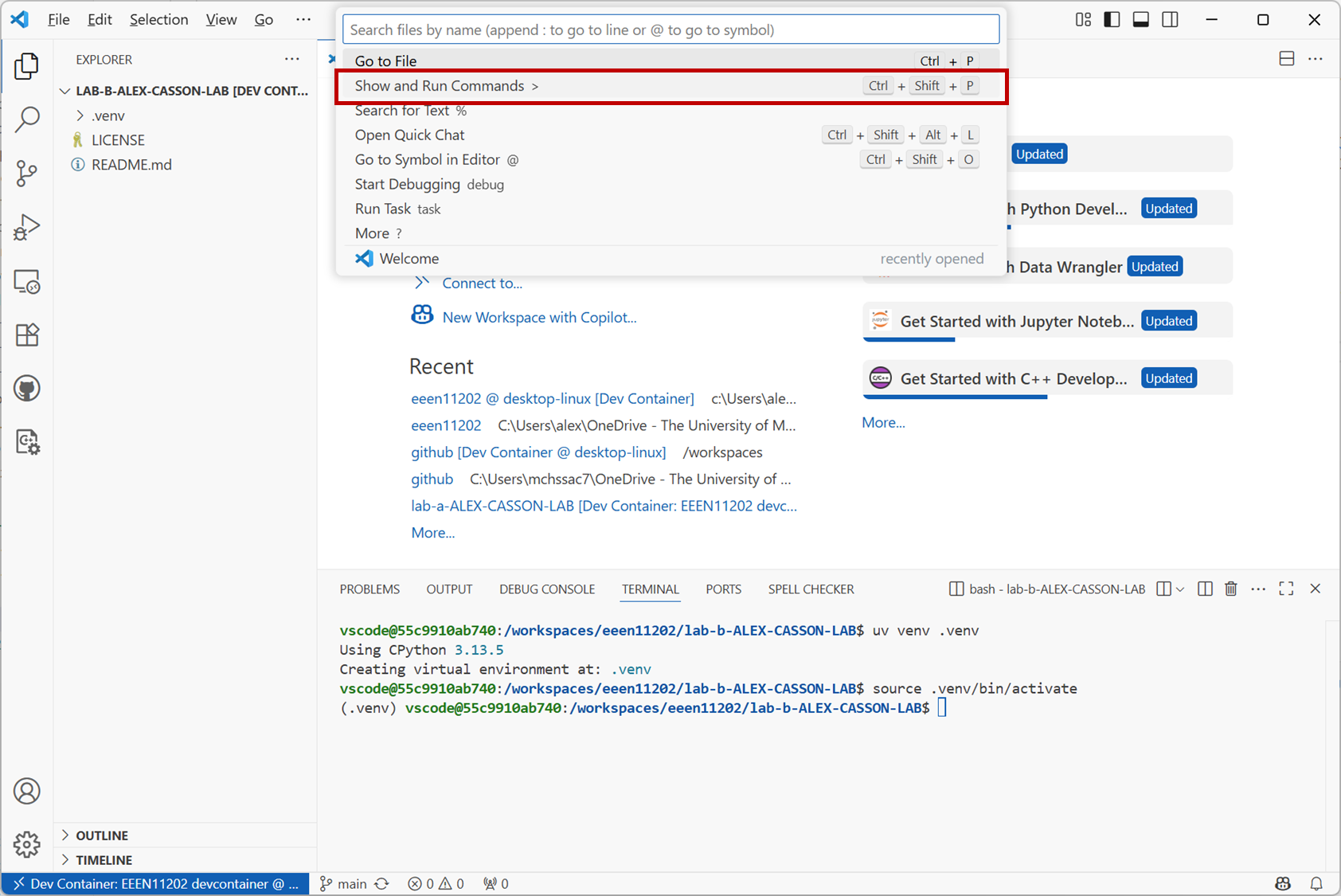

Screenshot of VSCode, software from Microsoft. See course copyright statement.¶

Search for Create: New Jupyter Notebook and click on this option. Or, scroll down and select it from the list of available commands.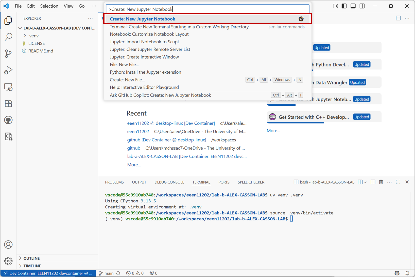

Screenshot of VSCode, software from Microsoft. See course copyright statement.¶

This opens a blank file, like that shown below.

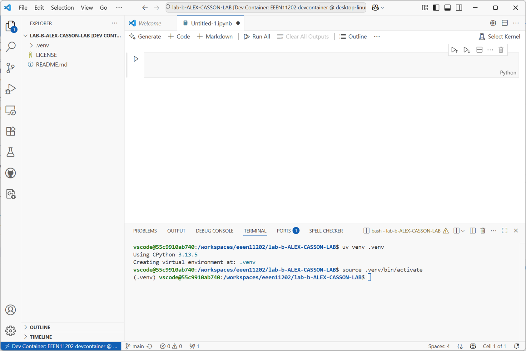
Screenshot of VSCode, software from Microsoft. See course copyright statement.¶

Save this to give it a name by clicking on File / Save As.... Pick any name that you would like. Make sure you save it in your lab_b folder.
Copy and paste the code below into a cell and run the cell. To do this, you may need to tell VSCode which Python virtual environment you want to use, in which case you should select .venv, the one we made in the previous part of the lab.
```
# Example for loop
mult = 11
lim_low = 0
lim_high = 5
for i in range(lim_low, lim_high):
    print(i * mult)
```
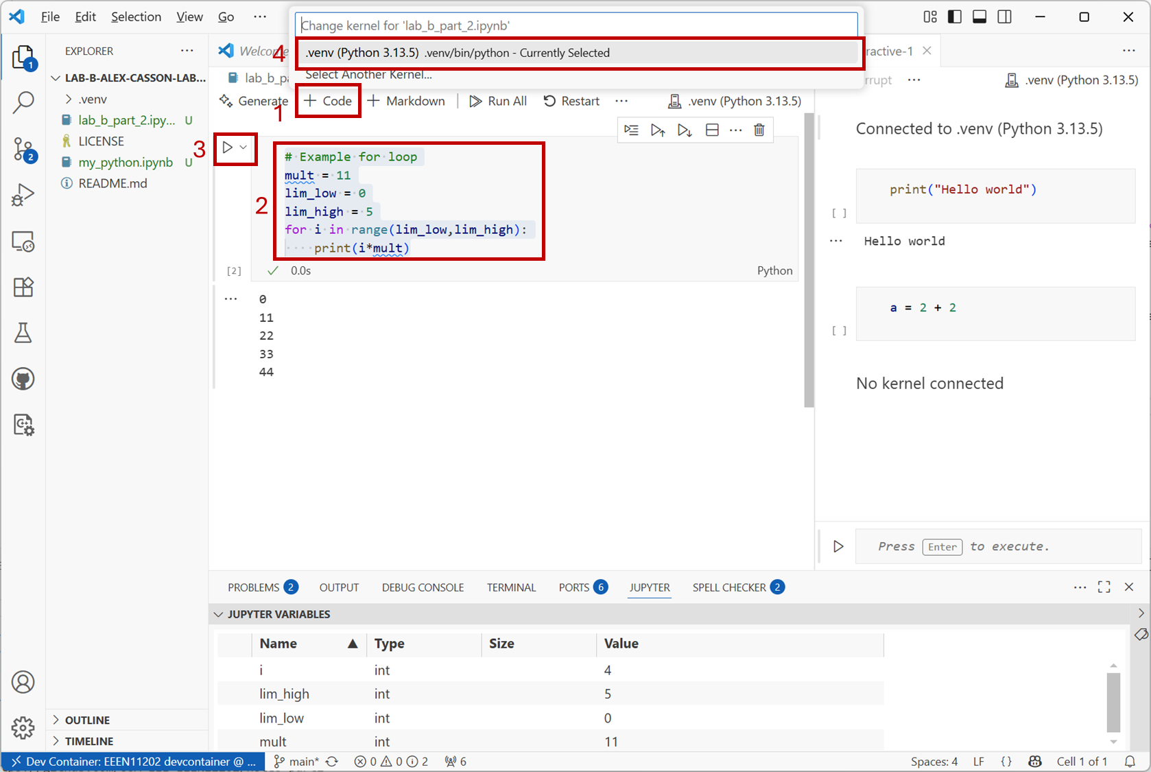
Screenshot of VSCode, software from Microsoft. See course copyright statement.¶

Notice how print(i * mult) is indented. This is how Python determines which parts of the code belong to the for loop.

Does the code do as you would expect? Ask a demonstrator to help explain the operation if it would be useful.

Solution

This code will display the numbers 0, 11, 22, 33, and 44.

lim_low is 0, and lim_high is 5. range(lim_low, lim_high) makes a list of numbers between these, i.e. 0, 1, 2, 3, and 4. 5 is the stopping point, this isn’t included. for is a loop which goes through each of these numbers in turn, putting them in the variable i. The code then carries out the multiplication i * mult.

Even in this simple example, there are no hard coded values. It’s tempting to write range(0, 5) or similar. However, this can give very fragile code. If we want to use the 5 somewhere else in the code as well as here, it’s better to put the number in a variable and use the variable everywhere. That way, if the number changes at some point in the future the new value will automatically be used everywhere that the variable is used.
Add a new Markdown cell by clicking on the + Markdown button.

Enter the text below in the the cell that’s made. When you’ve finished editing, click on the ✓ button (the Stop Editing Cell button).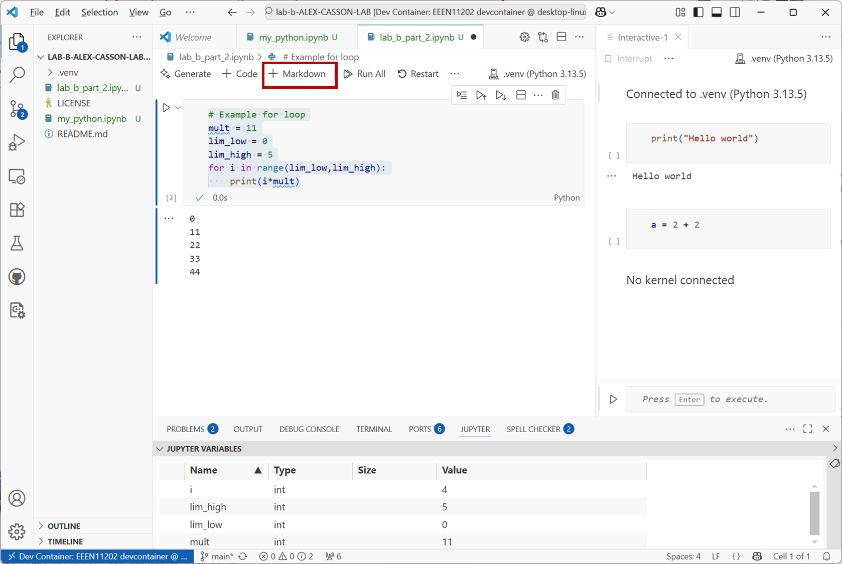

Screenshot of VSCode, software from Microsoft. See course copyright statement.¶
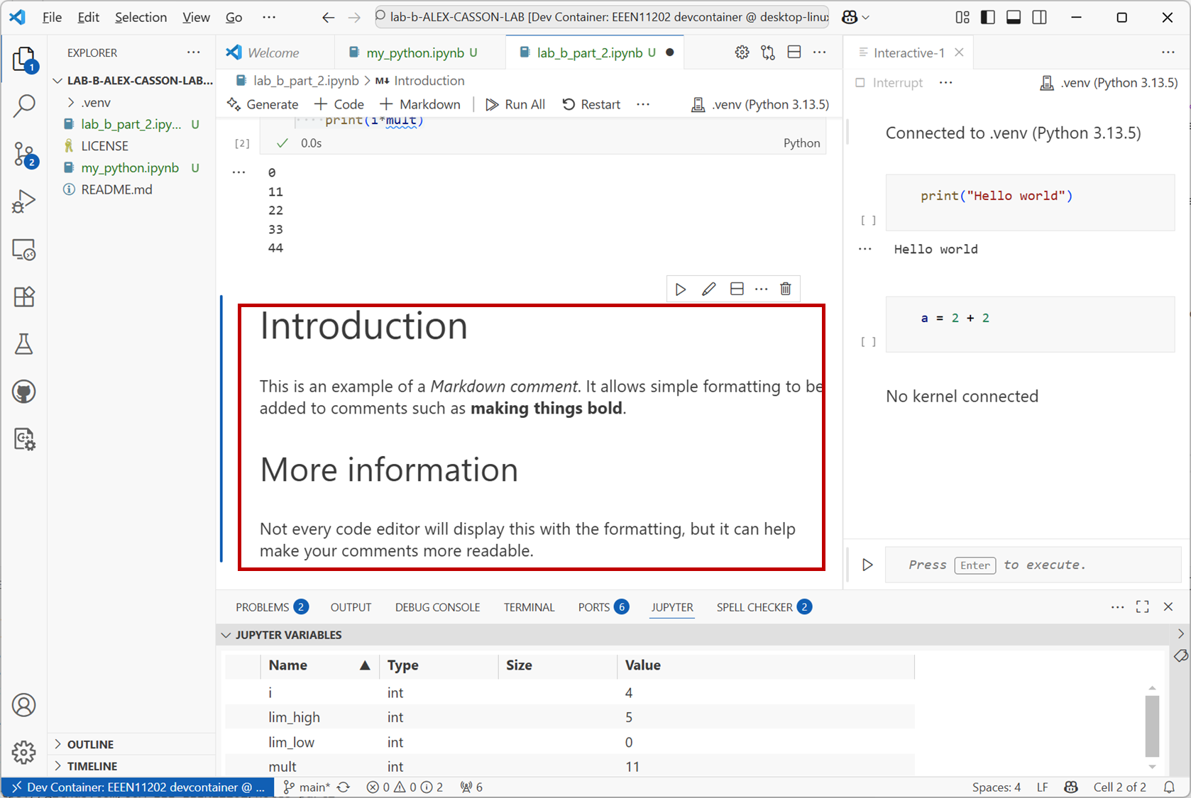
```
# Introduction
This is an example of a *Markdown comment*. It allows simple formatting to be added to comments such as **making things bold**.

## More information
Not every code editor will display this with the formatting, but it can help make your comments more readable.
```
This is a comment, but as it’s flagged as being in a markdown cell VSCode has displayed it with formatting. Markdown is a simple way of taking plain text, and indicating which parts should be displayed with some formatting. You can find a full list of Markdown formatting options at Markdown Cheatsheet.

Screenshot of VSCode, software from Microsoft. See course copyright statement.¶

Not every code editor will display the text with the formatting, some will just display the text. Nevertheless, it’s a nice feature for adding emphasis or structure to your comments.

2.3.2.2. Modelling sine waves¶

In Electronic Engineering it’s very common that we work with sine waves. Mathematically, this is $V_{out}(t) = A \sin (2\pi f t)$ where $A$ is the amplitude, $f$ is the frequency of the wave in Hz, and $t$ is the time in seconds. This is known as a time series, as to see a sine wave we need to know the value of $V_{out}(t)$ at multiple different points in time, not just at one time.

Make a new cell and copy and paste the below into it.
```
# Make a sine wave
sample_start = 0
sample_stop = 100
t = range(sample_start, sample_stop)  # interpret as representing 1 s, 2 s, 3 s, ...
```
t will produce numbers 0, 1, 2, 3, up to sample_stop-1, and we as humans can think of these as representing time points, 0 second, 1 second, and so on.

Danger

There is a better way of doing this! The range function can only make integer time points (1 s, 2 s, 3 s, and so on). In Lab E we’ll use numpy arrays to do the same thing, with a number of other benefits. Using numpy is probably nearly always what you should actually do. We’ve included this example here to give an Electronic Engineering example early on, even if you learn better ways of achieving the same functionality later.

To implement the equation $V_{out}(t) = A \sin (2\pi f t)$ we need a $\sin$ function, and the number $\pi$. These are available in the Python math module. This is the part of the Python standard library. This is a built-in part of Python, but you need to explicitly add it to your code with the import function.

Add the code below to your function.
```
# Calculate the sine wave
import math

A = 1  # Volts
f = 0.1  # Hz
v_out = [A * math.sin(2 * math.pi * f * time) for time in t]
```
math.pi contains 3.1415…, the value of $\pi$. Here there is a small for loop which goes through each value in t, puts it in a list called time, and calculates the value of v_out for each value of time.

Run the code. In the variable explorer you should be able to see a range of values for time and v_out.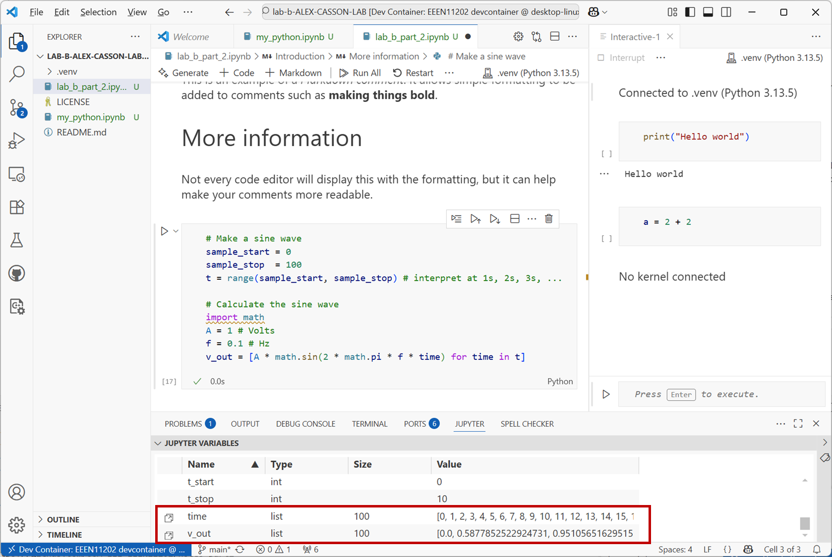

Screenshot of VSCode, software from Microsoft. See course copyright statement.¶
The variable explorer is very useful for examining the results of calculations, checking that variables contain the correct thing, and so on. It has more functionality, but we need to install a Python module called Pandas to add this functionality. Pandas is very widely used, but it’s not part of the standard library so we need to ensure it’s in the virtual environment by installing it ourselves.

Click on the Terminal tab in VSCode. It should look like the below. You should see that (.venv) is present, indicating the virtual environment we’re working in is active. (If not, make sure the terminal is in the lab_b folder, and then activate the .venv with source .venv/bin/activate.) You should also see that the command prompt looks like $, indicating that this is the computer’s terminal, not a Python terminal (which would be >>>).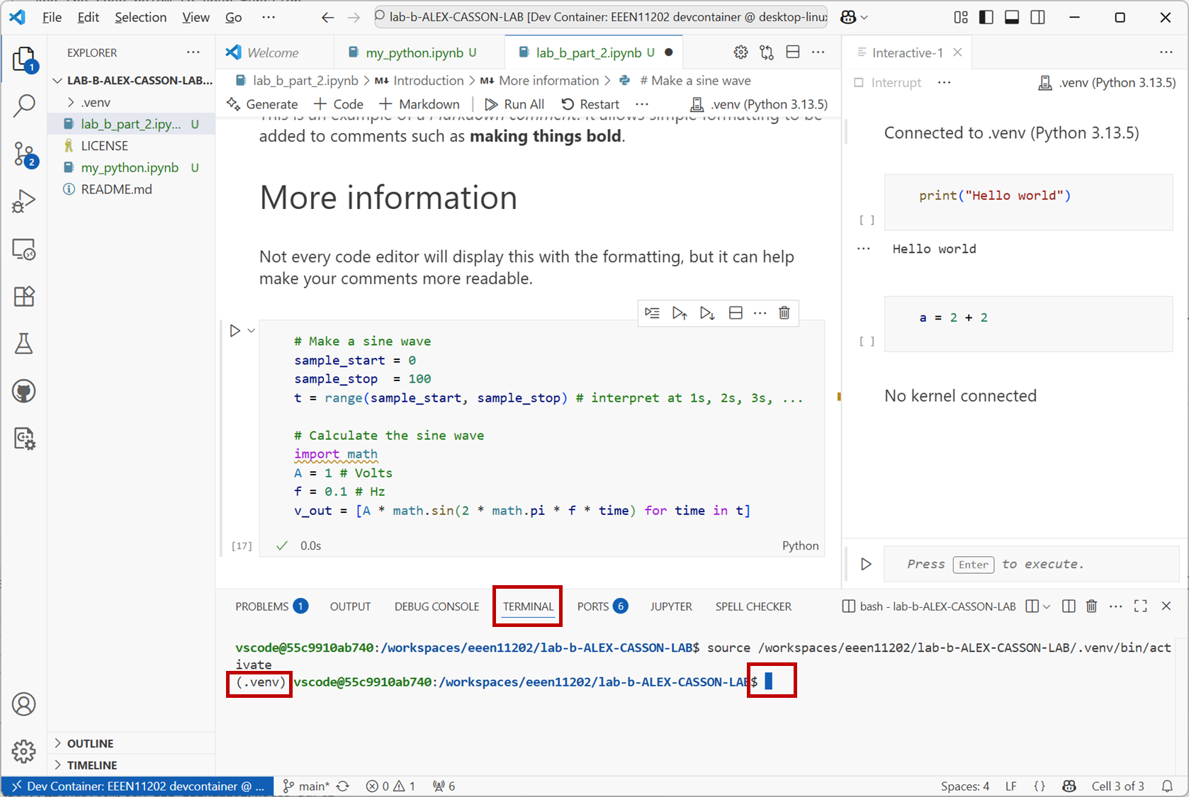

Screenshot of VSCode, software from Microsoft. See course copyright statement.¶

At the computer terminal enter
```
uv pip install pandas
```
This will install Pandas into the virtual environment. It may take a minute. It’s only been installed in the virtual environment that’s currently active. When you make or use a new or different virtual environment, you may need to install it again. (Which is one of the aims of using virtual environments, we could install different versions of Pandas in different virtual environments if we wanted to.)

Aside

In the next lab we’ll look at how to list dependencies in a file so we have a list of what needs to be installed in order for our code to run.

VSCode won’t pick up the installation of Pandas automatically if you install it while VSCode is running. Click on the Restart button, and then Restart again to confirm. This restarts the Python kernel so that it will pick up any changes to the virtual environment.

Then press Run All to re-run the code and it will be picked up.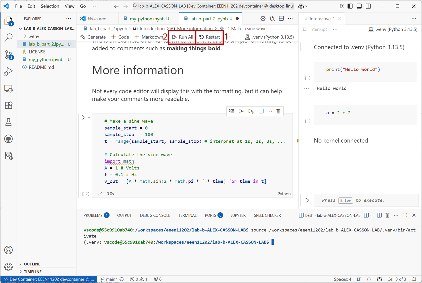

Screenshot of VSCode, software from Microsoft. See course copyright statement.¶

Click on the Jupyter tab in VSCode. Then double click on v_out to open a more detailed view of what’s stored in the variable. (You may need to scroll down in the variable explorer to see v_out.) You should have a view similar to the below. Check some of the values using your calculator to check that they’re what you expect.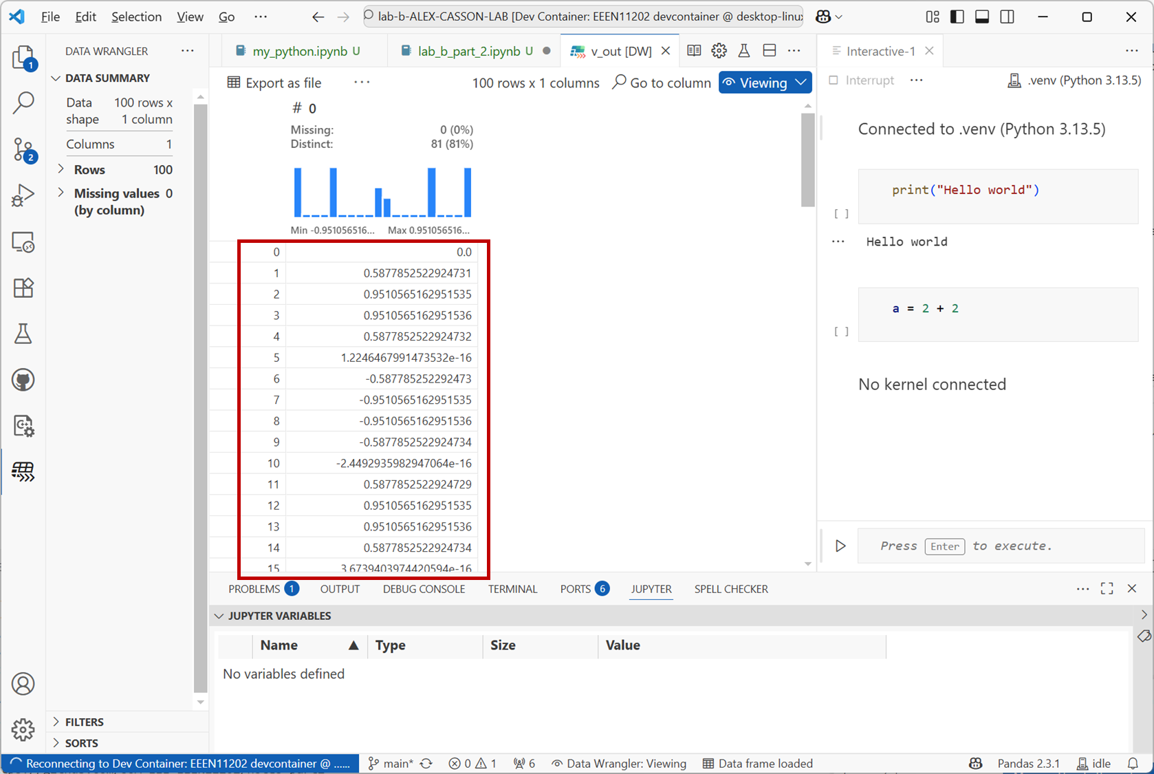

Screenshot of VSCode, software from Microsoft. See course copyright statement.¶
For this example, probably an even better way to exploring the data is to plot it. Again, we need internal an external module to do this.

Note

We’re going to look at data visualization more in Lab F. There are lots of options beyond what we’re going to look at here. This example is just something to get started with.

At the computer terminal enter
```
uv pip install plotly jupyterlab anywidget
```
Then restart the Python kernel as before.

In your code cell add
```
# Plot the sine wave
import plotly.express as px

fig = px.line(x=t, y=v_out, labels={'x': 'Time [s]', 'y': 'Voltage [V]'})
fig.show()
```
This adds a module called plotly to your code, and asks it to plot t on the x-axis and v_out on the y-axis. When you run the code, it will display a plot similar to the below. There are a number of controls to zoom in and out, and similar. Explore these.

Try changing the values of A and f to see how the plot changes. In particular, try f = 0.01 and f = 10. Do you see what you expect?

Solution

When f = 0.01 you see a sine wave as you expect. It’s quite a low frequency sine wave, and so we don’t see many oscillations present in 100 seconds. When f = 10 we don’t see a sine wave. f = 10 means were expecting 10 oscillations per second. However our time points are only at 0 s, 1 s, 2 s, and so on. (We’re sampling at 1 Hz.) We’re not sampling quickly enough to see the oscillations. Indeed in this case we’re sampling so slowly that we get a very strange shape indeed.

You’ll learn about the Nyquist theory later in your degree. In general, we need the sampling frequency to be at least twice as fast as the highest frequency we want to plot. (This is nothing to do with Python, it applies to all cases of plotting a waveform.) If we’re sampling at 1 Hz, the largest f we can have is 0.5 Hz. In practice, the ratio needs to be more like 10-30 times the highest frequency to get a good plot.

Set
```
A = 1  # Volts
f = 0.1  # Hz
```
again and re-run the code before proceeding.
We can use an if statement to check whether a condition is true or not. Make a new cell and enter to the code
```
# Find zero crossings
for i, v in enumerate(v_out):
    if v == 0:
        print("Zero crossing at time:", i)
```
This is intended to display the times at which the sine wave crosses zero. It passes through each value in v_out, puts it in a temporary variable called v and checks whether this is equal to 0.

Run the code. Does it display what you expect? If not, why not?
Solution

In the plot we can clearly see the sine wave crossing 0. Have a look in the variable explorer however. You’ll see it’s only 0 at the time point 0. After this, it gets very close to 0, for example $1.22 \times 10^{-16}$. This is a very small number, but it’s not exactly 0! The == 0 is checking for exactly zero. We’re seeing the impact of floating point numbers. Rather than getting exactly 0 were getting a little bit of rounding error. This is negligible in any practical sense (if this was a voltage we’ve measured from a circuit, it’s very hard to measure $1.22 \times 10^{-16}$ Volts. However it means that our code doesn’t do what we want in this case. Try
```
# Find zero crossings
for i, v in enumerate(v_out):
    if v < 1e-15 and v > -1e-15:
        print("Zero crossing at time:", i)
```
This is a bit more generous in its checking and should work as you want.

2.3.2.3. Circuit analysis examples¶

Python can also do complex maths, as we commonly need for circuit analysis. There is a module cmath in the standard library which adds functions for working with complex numbers. Make a new cell and enter the code below.
```
# Examples of complex sums
import cmath

# Simple sums
a = 1 + 1j
b = 2 * cmath.exp(4j)
c = a * b

d = abs(c)
e = cmath.phase(c)
g = c.real
h = c.imag
k = c.conjugate()
```
a is $1 + 1j$. b is $2 e^{4j}$. That is, a is in Cartesian form, and b is in polar form. This is fine. Python can work with either, and automatically convert between the two as needed. You can enter a complex number in whichever form is easiest for you. There are then built in functions to find the magnitude (the abs function), and then for the phase, the real part, the imaginary part, and the complex conjugate. Run the code and view these results in the variable explorer and check they are what you expect.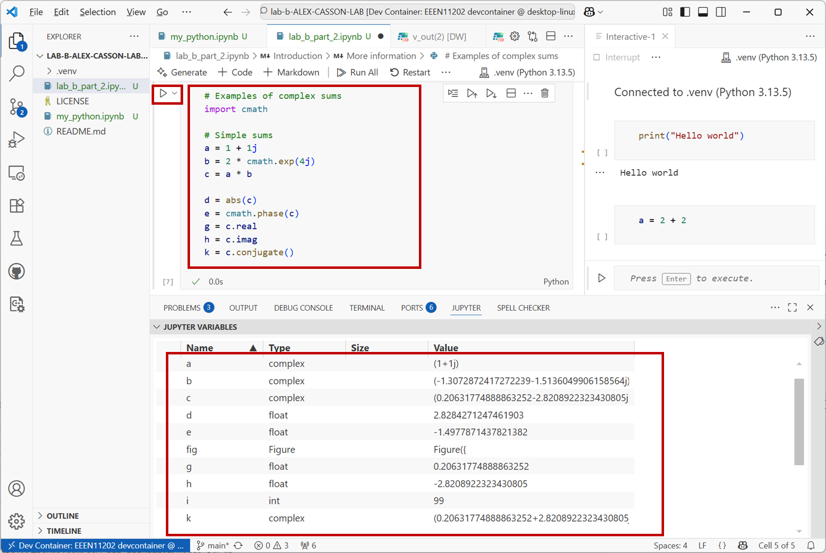

Screenshot of VSCode, software from Microsoft. See course copyright statement.¶

2.3.2.4. Tracking components¶

The examples so far have focused on processing numbers. Python can process text as well.

Make a new cell and enter the code below.
```
# Make bill of materials
r1 = {"component_number": 1, "type": "resistor", "value": 1000, "units": "ohm"}
r2 = {"component_number": 2, "type": "resistor", "value": 10e3, "units": "ohm"}
c1 = {"component_number": 3, "type": "capacitor", "value": 1e-6, "units": "F"}
bom = (r1, r2, c1)
```
This makes a simple Bill Of Materials (BOM), for example for if we were making a circuit. The BOM is stored in a tuple. A tuple is immutable so we can’t accidentally change the components. The details on each component are stored in a dictionary. This lets us store a range of information about the component, both text and numbers.

We can then start to automatically process this list. Add the code below to the cell and run it.
```
# Count components in the BOM
resistors = 0
capacitors = 0
for component in bom:
    if component["type"] == "resistor":
        resistors += 1
    elif component["type"] == "capacitor":
        capacitors += 1
    else:
        print("Unexpected component. Was expecting only resistors or capacitors")
print(f"{resistors} resistors and {capacitors} capacitors are in the BOM.")
```
This code combines a for loop with an if statement to count the number of resistors and capacitors in the BOM. Make sure you understand how this works before you move on. Note the different levels of indentation to show which code belongs to which part of the structure.

The syntax in print(f"{resistors} resistors and {capacitors} capacitors are in the BOM.") is known as an f-string. Notice that the string starts f". In an f-string, items in curly brackets {} are replaced with their values. So with {resistors} the value of the variable resistors is displayed rather than the word resistors.

2.3.2.5. Further questions¶

Resistors in parallel add following the equation

\[\frac{1}{R_{T}} = \frac{1}{R_1} + \frac{1}{R_2} + \frac{1}{R_3} + \ldots\]

where $R_{T}$ is the total resistance and $R_{1}$ (and similar) are the value of each individual resistor being connected in parallel.

You are given 10 resistors connected in parallel, values: 10 k ${\Omega}$, 20 k ${\Omega}$, 30 k ${\Omega}$, 40 k ${\Omega}$, 50 k ${\Omega}$, 60 k ${\Omega}$, 70 k ${\Omega}$, 80 k ${\Omega}$, 90 k ${\Omega}$, and 100 k ${\Omega}$. Write a code cell to calculate $R_{T}$, the total effective resistance present. View your calculated value in the variable explorer.
Solution
```
# Calculate the total resistance
r_values = range(10, 100, 10)  # kOhm values
r_intermediate = [1 / r for r in r_values]  # broken into two lines for readability
r_t = 1 / sum(r_intermediate)  # kOhm values
```
A potential divider is made when the output voltage is taken from a point between two impedances, labelled $Z_{1}$ and $Z_{2}$ in the figure below.

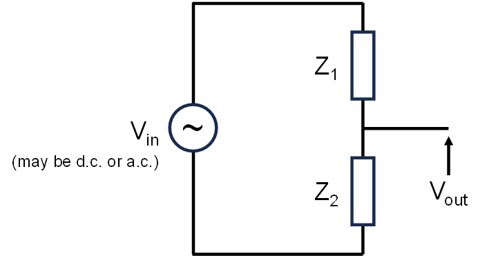
Recall from your circuit analysis course that the relationship between the input and output voltages is given by

\[V_{out} = \frac{Z_{2}V_{in}}{Z_{1} + Z_{2}}\]

If both impedances are resistors, $Z_{1}$ and $Z_{2}$ will be real numbers. Use the Python code below to calculate the output voltage for the case when:
- $V_{in}$ = 10 V (d.c.).
- $Z_{1}$ = 1 k ${\Omega}$.
- $Z_{2}$ = 10 k ${\Omega}$.
```
# Potential divider example
v_in = 10
z1 = 1  # kOhm
z2 = 10  # kOhm
v_out = (z2 * v_in) / (z1 + z2)  # Volts
```
$Z_{1}$ is kept as a resistor of value 1 k ${\Omega}$, and $Z_{2}$ is replaced by a capacitor.

A capacitor has an impedance (in ${\Omega}$)

\[Z = \frac{1}{j\omega C}\]

where $\omega$ is the angular frequency

\[\omega = 2\pi f\]

$f$ is the frequency of the a.c. source in Hz, and $C$ is the capacitance in Farads. When considering the impedance of the capacitor (not its capacitance in Farads, its impedance in Ohms) the same potential divider equation as in Step 2 is valid without modification.

Make a copy of your code from Step 2. Change the definition of $Z_{2}$ to be a complex number:
```
z2 = 1 / (1j * w * c)
```
where w is the angular frequency and c is the value of the capacitance. Make suitable variables for these, assuming a capacitor of value 1 nF and frequency of 160 kHz.

Modify the v_in in your code to be an a.c., sinusoidal signal with a frequency of 160 kHz, phase of 0, and amplitude of 5 V. Mathematically, you can represent this as a phasor, that is, a complex exponential. Recall that from your circuit theory you would represent such an input as $5e^{j\omega}$ where $\omega = 2\pi \times 160,000$.

In Python you can represent this as
```
v_in = 5 * cmath.exp(1j * 2 * math.pi * 160000)
```
(assuming that you already have import cmath and import math in your code).

With these two changes, find the magnitude and phase of the output voltage, $V_{out}$. You can do this with the abs and cmath.phase commands.
Solution
```
import cmath
import math

# Potential divider where z2 is a capacitor
f = 160000  # Hz
w = 2 * math.pi * f  # rad/s

v_in = 5 * cmath.exp(1j * w)

z1 = 1  # kOhm
c = 1e-9  # Farads
z2 = 1 / (1j * w * c)

v_out = (z2 * v_in) / (z1 + z2)  # Volts
vout_mag = abs(v_out)
vout_phase = cmath.phase(v_out)
```
Using your code from above, change the frequency of the input (and the one used in the z2 equation). Pick some frequency values and see how the magnitude of $V_{out}$ changes. (We suggest making quite big steps in frequency, go up and down from 160 kHz by factors of 10, and then 100.)

Based on the results of your simulation, does this circuit act as a high pass filter (where low frequency signals are blocked but high frequency signals passed through) or a low pass filter (where low frequency signals are passed through but high frequency signals are blocked)?

Solution

Low pass filter.