4.2.1. Numpy examples¶

4.2.1.1. Initial setup for the Lab¶

In the VSCode terminal enter:
```
cd /workspaces/`ls /workspaces`/lab-e
uv init .
```
Remember to enter these one at a time, not both together.

This will make a new Python project in the current folder. It will be named automatically after the folder name.

To analyze these lines:
- cd /workspaces/`ls /workspaces`/lab-e makes sure we are working in the lab-e folder.
- uv init . is the interesting command. This actually sets up our virtual environment.
The above will make the a pyproject.toml file, a main.py file, and a number of others.
Add some structure to your code folder by entering the commands:
```
mkdir tests docs
mv main.py src
uv run src/main.py
touch tests/__init__.py
```
- Here we’ve moved main.py into the src folder. You’ll see that the src folder already contains some code that we’ve written for you.
- We’ve made a tests folder for any tests that we might want to write later, and a docs folder for any documentation. We won’t ask you to put anything into these as part of the lab instructions, but you might want to write some tests for your code to check that it’s working!
- In the files that were downloaded from Git automatically, you’ll also see there’s a folder called data. This contains some files that we’ll analyze during the lab.
Install the required dependencies for this lab by entering the command:
```
uv add numpy scipy pandas plotly
```
Run
```
uv run src/main.py
```
to make sure the virtual environment is built.
When you open a Python file, make sure that the correct Python virtual environment is activated. See the instructions in Lab D if you’re unsure.

4.2.1.2. Numerical analysis in Python¶

Make a new Python file with any suitable name. Put it in your Lab E src folder.
In this file, copy the code below and run it. We suggest putting a breakpoint on the return statement on Line 13 so you can view the results, or you can inset logging commands if you prefer.
```
import numpy as np


def vector_and_matrix_multiplication():
    # Define vectors
    v1 = np.array([1, 2, 3])
    v2 = np.array([4, 5, 6])

    # Perform vector-matrix multiplication
    r1 = np.dot(v1, v2)  # dot product
    r2 = np.cross(v1, v2)  # cross product

    return


if __name__ == "__main__":
    vector_and_matrix_multiplication()
```
The view in the debugger will be like the below.

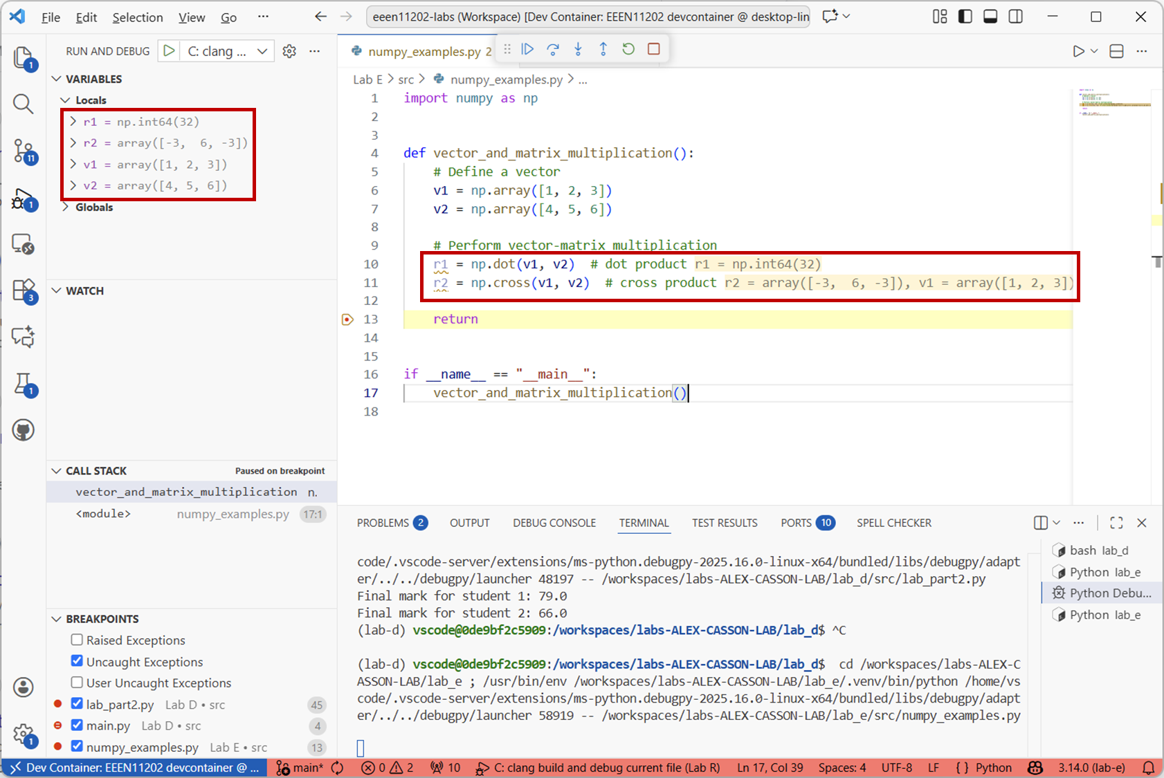
Screenshot of VSCode, software from Microsoft. See course copyright statement.¶

From your Maths courses you should remember multiplying vectors, where you can use the dot product to get a scalar result, or the cross product to get another vector. numpy makes this very easy.

To analyze the code briefly:
- import numpy as np adds the numpy library to the code. Functions have a namespace, essentially an address to the function so that functions with the same name don’t conflict with one another. By importing numpy as np, we can use the shorter np prefix to access functions in the numpy library.
- np.array([...]) creates a numpy array. These are 1D arrays, and so they are representing vectors. np.array([...]) is not one of the built in data types in Python, numpy has added it.
- np.dot() and np.cross() are then the numpy functions for calculating the dot product and cross products respectively.
To work with matrices, we can make 2D arrays. Add the code below to the vector_and_matrix_multiplication() function, and run it again.
```
# Define matrices
m1 = np.array([[1, 2, 3],
               [4, 5, 6],
               [7, 8, 9]])
m2 = np.array([[9, 8, 7],
               [6, 5, 4],
               [3, 2, 1]])

# Perform matrix multiplication
r3 = m1 @ m2  # matrix multiplication
r4 = np.matmul(m1, m2)  # alternative method
```
You should see the result of the matrix multiplication in the debugger view.

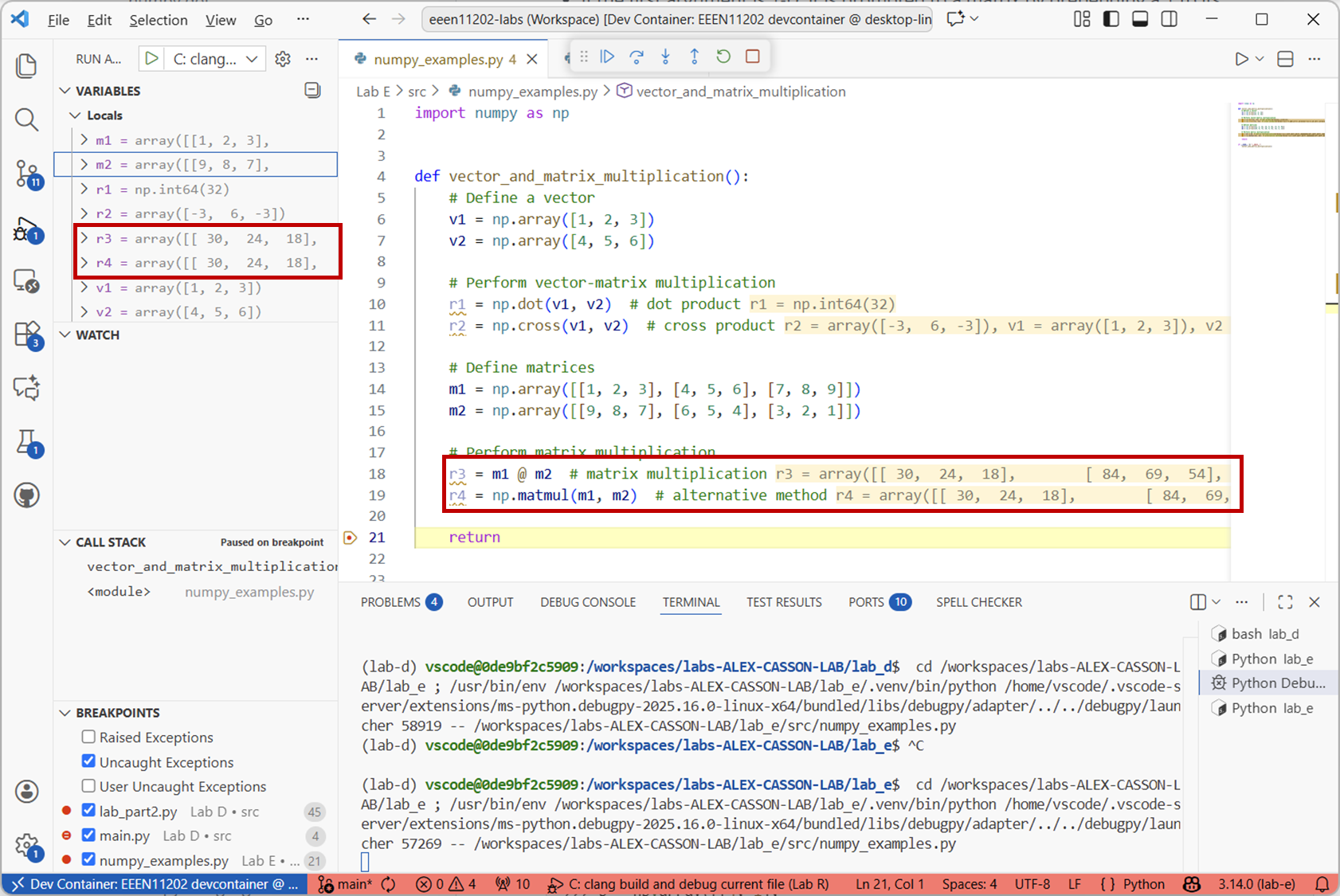
Screenshot of VSCode, software from Microsoft. See course copyright statement.¶

This defines two 3x3 matrices, and then performs a matrix multiplication. There are two different syntaxes, both of which give the same result. @ is just a short hand as multiplying matrices is a common thing to want to do.
In many engineering applications, we need to solve systems of linear equations. These are equations like the below. The aim is to find the value of \(x\).

\[Ax = b\]

where for example

\[ \begin{align}\begin{aligned}\begin{split}A &= \begin{bmatrix} 1 & 2 & 3 \\ 1 & 0 & 1 \\ 3 & 1 & 3 \end{bmatrix}, \\\end{split}\\\begin{split} b &= \begin{bmatrix} 5 \\ 3 \\ 3 \end{bmatrix}\end{split}\end{aligned}\end{align} \]

By searching the Internet, asking AI, or similar, add code to your vector_and_matrix_multiplication() function to work out the value of \(x\) for the \(A\) and \(b\) given above.
Solution
```
# Solve linear equations
A = np.array([[1, 2, 3], [1, 0, 1], [3, 1, 3]])
b = np.array([5, 3, 3])
x1 = np.linalg.solve(A, b)
x2 = np.linalg.inv(A) @ b  # alternative method
```
Again solving linear systems is quite a common thing to do, and so it’s got it own dedicated function in numpy, np.linalg.solve(). An alternative method is to calculate the inverse of \(A\) using np.linalg.inv(), and then multiply it by \(b\). Both methods give the same result.
What is the value of \(x\) when

\[ \begin{align}\begin{aligned}\begin{split}A &= \begin{bmatrix} 2 & 1 & 0 & 0 & 0 \\ 1 & 2 & 1 & 0 & 0 \\ 0 & 1 & 2 & 1 & 0 \\ 0 & 0 & 1 & 2 & 1 \\ 0 & 0 & 0 & 1 & 2 \end{bmatrix}, \\\end{split}\\\begin{split} b &= \begin{bmatrix} 1 \\ 1 \\ 1 \\ 1 \\ 1 \end{bmatrix}\end{split}\end{aligned}\end{align} \]

Solution

\[\begin{split}x &= \begin{bmatrix} 0.5 \\ 0 \\ 0.5 \\ 0 \\ 0.5 \end{bmatrix}\end{split}\]

4.2.1.3. Simulating signals in Python¶

In your Lab E src folder we’ve placed a Python file called sine_plotting.py. Open this file.

It contains a function called make_sine_wave(), shown below. It’s a minor variant on the code we introduced in Lab B.
```
def make_sine_wave():
    """
    Make a sine wave signal
    TO DO: replace range with a numpy array

    Returns: t: time samples
    v_out: voltage samples
    """
    sample_start = 0
    sample_stop = 100
    A = 1  # Volts
    f = 0.1  # Hz
    t = range(sample_start, sample_stop)  # interpret as representing 1 s, 2 s, 3 s, ...
    v_out = [A * math.sin(2 * math.pi * f * time) for time in t]
    return t, v_out
```
This code is not ideal, because range() can only generate whole numbers, which we have to interpret as representing seconds (1 s, 2 s, 3 s, …). Now we can make numpy arrays that can have numbers that we like. Also, it uses a for loop to calculate the value of sin at each time sample. Numpy can do this sort of operation much more efficiently without needing a loop.
In sine_plotting.py there is also a function called make_sine_wave_numpy(). This is a version of the same function, but using numpy arrays. The code is given below.
```
def make_sine_wave_numpy(A, f, start, stop):
    """
    Make a sine wave signal
    Returns: t: time samples
    v_out: voltage samples
    """
    step = 1 / (f * 30)
    t = np.arange(
        start, stop, step
    )  # interpret as representing 1 s, 2 s, 3 s, ...
    v_out = A * np.sin(2 * np.pi * f * t)
    return t, v_out
```
The key changes are:
- t is now made using np.arange(), which is similar to range(), but can have any step size. Here the step size is set to 30 samples per cycle of the sine wave, which makes a nice plot whatever value of f is used.
- math.sin() has been replaced with np.sin(). This can take a numpy array as the input, and will calculate the sin of each element in the array automatically. We don’t need a for loop to cycle through every element in the array.
In sine_plotting.py there is also a function called plot_sine_wave(). Add code to if __name__ == "__main__": to make a sine wave of amplitude 1 V, frequency 0.1 Hz, from time 0 s to 50 s, and then plot it. Do this using both make_sine_wave() and make_sine_wave_numpy() to see the difference.
Solution
```
if __name__ == "__main__":
    # Put plotting code below here
    A = 1  # Amplitude in V
    f = 0.1  # Frequency in Hz
    start = 0  # Start time in s
    stop = 50  # Stop time in s
    t, v_out = make_sine_wave(A, f, start, stop)
    do_plots(t, v_out)
    t, v_out = make_sine_wave_numpy(A, f, start, stop)
    do_plots(t, v_out)
```
You should see plots like the below, where the bottom one is made using numpy.

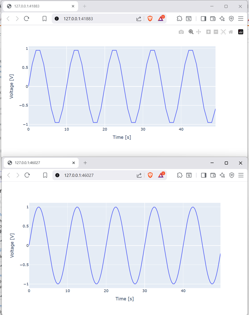
Screenshot of a web browser, software from Brave. See course copyright statement.¶
Experiment with different values of A and f to see the different signals produced. If you make the frequency f very high you might want to decrease the stop time to see just a few cycles of the sine wave.
An important feature of numpy is that it can operate on whole arrays at once. This is called vectorization. It saves us from having lots of for loops which, by definition, need to be run multiple times and so can make the code slower to run.

Add the below to your code
```
# Settings for both sine waves - both need the same time base
start = 0
stop = 1
fs = 500  # sampling frequency in Hz
time = np.arange(start, stop, 1 / fs)

# Make sine wave 1
A1 = 1
f1 = 10
v1 = A1 * np.sin(2 * np.pi * f1 * time)

# Make sine wave 2
A2 = 0.4
f2 = 50
v2 = A2 * np.sin(2 * np.pi * f2 * time)

# Make final sine wave
vo = v1 + v2
do_plots(time, vo)
```
We can just add the two arrays, v1 and v2, together directly. Numpy will automatically add the corresponding elements in each array together to make a new array, vo. This is much simpler than needing to write a for loop to do the addition element by element. We just need to make sure that the arrays have the same number of elements in them so that the addition makes sense.
You should see a plot like the below. This is a 10 Hz sine wave with a smaller 50 Hz sine wave superimposed on top of it. 50 Hz is the mains frequency in the UK, so this sort of trace could be representing a low frequency signal with some mains interference on top of it. In the lab, it’s quite common that we see 50 Hz interference in our measurements.

Screenshot of a web browser, software from Brave. See course copyright statement.¶
We can make this signal model more realistic still by adding some random noise to it. Numpy provides a number of functions for this. We’ll use np.random.normal() to generate white Gaussian noise.

Add the below code to your file.
```
# Add random noise
noise_mean = 0
noise_std = 0.2  # standard deviation of the noise, the peak-to-peak will be about 6 times this
noise = np.random.normal(noise_mean, noise_std, size=vo.shape)
vo_noisy = vo + noise
do_plots(time, vo_noisy)
```
This generates random noise with a mean of 0 and a standard deviation of 0.2, and then adds this to the signal. You should see a plot like the below.

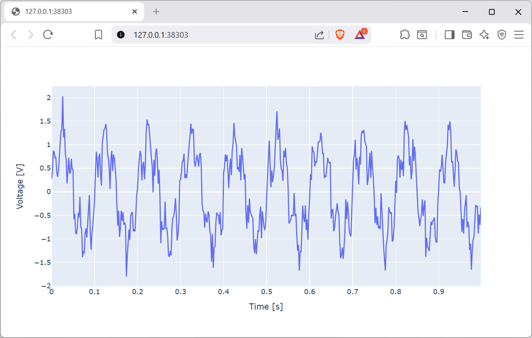
Screenshot of a web browser, software from Brave. See course copyright statement.¶
Let’s try another example. Using the time vector ts defined below
```
start = 0
stop = 1
fs = 500  # sampling frequency in Hz
ts = np.arange(start, stop, 1 / fs)
```
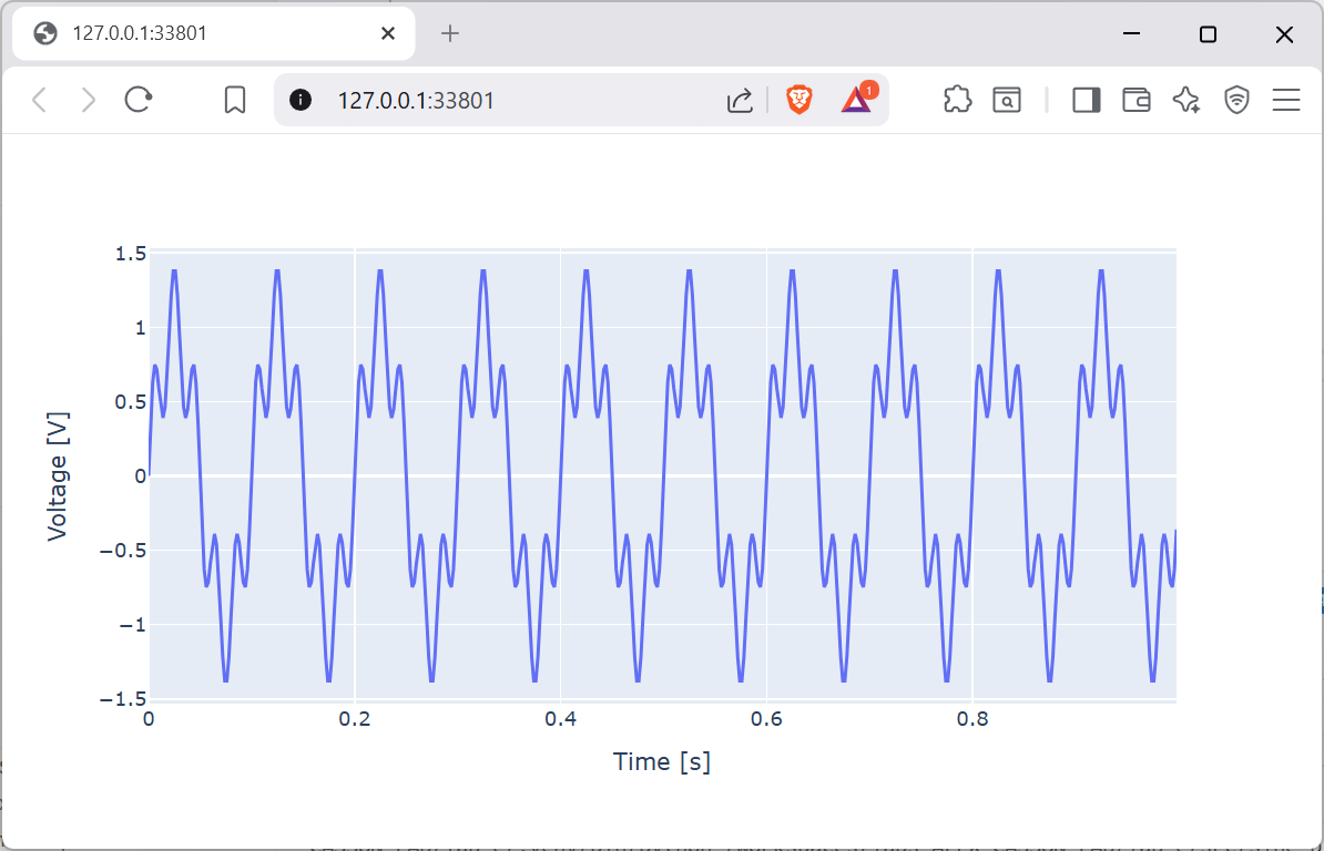
and f = 10, make a signal that follows the equation below. Run your code for different values of \(n\). What does the signal look like as the value of \(n\) gets bigger?

\[v(t) = \frac{4}{\pi} \sum_{k=1}^{n} \frac{1}{(2k-1)}\sin((2k-1) \times 2 \pi f t)\]
Solution
```
f = 10  # frequency in Hz
n = 10  # number of harmonics to add
vs = np.zeros_like(
   ts
)  # initialize v to be an array of zeros the same shape as t, lets us just add values to this in the for loop
for k in range(1, n + 1):  #  range doesn't include stop value
   vs += (4 / (((2 * k) - 1) * np.pi)) * np.sin(((2 * k) - 1) * 2 * np.pi * f * ts)
vs = (4 / np.pi) * vs  # scale the final result
do_plots(ts, vs)
```
As more terms are added, the signal looks more and more like a square wave. (This is an example of a Fourier series which you’ll learn about in your Maths course. Briefly, any periodic signal can be approximated by adding together sine waves of different frequencies and amplitudes.)

Numpy doesn’t have a function to make square waves directly, but scipy does. You can use scipy.signal.square() to make square waves more easily than the above.

4.2.1.4. Array slicing¶

It’s common that we don’t want to work with an entire numpy array. It might have thousands, or millions of elements in it. An array can be sliced to access just a few elements in it. This uses square brackets [] and numbers to indicate which elements we want to access. A colon : is used to indicate a range of elements.

Make a time vector using the code below.

start = 0
stop = 1
fs = 500  # sampling frequency in Hz
ts = np.arange(start, stop, 1 / fs)

Work out the values of each of the below:
- ts[0]
- ts[1]
- ts[-1]
- ts[0:100]
- ts[-100:]
Solution
- ts[0] is the first element in the array, 0.
- ts[1] is the second element, 0.002.
- ts[-1] is the last element, 0.998.
- ts[0:100] is a new array containing the first 100 elements.
- ts[-100:] is a new array containing the last 100 elements. (If a number of either side of a colon : is omitted Python takes all the values to or from the end of the array.)