4.2.2. Scipy examples¶

Scipy provides lots of useful functions for scientific computing, such as analyzing signals. This forms the starting point for implementing signal processing, which is a very common topic in electronic engineering. For example, as we had the first part of the lab, most things that we measure in the lab are subject to interference and noise from other sources. Signal processing can help us filter and remove this noise.

4.2.2.1. Signal filtering example¶

In your Lab E folder you will see there is also a folder called data. Here we’ve put some files that contain pre-saved data for us. For example, this might be a recording we did in the lab using an oscilloscope or data acquisition system.

We’ve stored the data in Matlab format, with an extension .mat. This is a very dense data format that lets us store lots of data in a relatively small file size.

Aside

.mat format is a proprietary implementation of the open source hierarchical data format (HDF5). We could work with HDF5 files directly using the h5py library, but it’s easier to use the scipy.io functions that can read and write .mat files, and .mat files are widely used and inter-operable with open source tools.

Scipy has a function that can read these .mat files for us, called scipy.io.loadmat(). You can read its documentation online.
Start a new Python file in your Lab E src folder. Call it something like signal_filtering.py. Write a function that loads the file data/signal_data.mat, and extracts the time vector and signal vector from it, and then plots it.
- The variable names in the file are t for the time vector, and v for the signal vector.
- You might need to think about where the data file is located relative to your code file. In the solution below we’ve used the pathlib library to find this automatically, but you can just type in the address by hand if you prefer.
- Think about what type of variables you want to store your output in. scipy.io.loadmat() will load the data into a dictionary, so you probably want to extract the variables from this dictionary and put them in numpy arrays.
Solution
```
import pathlib
from os.path import join as pjoin

import numpy as np
import plotly.express as px
import scipy.io as sio
from scipy import signal


def load_signal_from_matfile():
    # Get the path to the .mat file
    # This uses pathlib to automatically get the folder where this script is located and navigates from there
    script_folder = pathlib.Path(__file__).parent.resolve()
    data_dir = pjoin(script_folder, "../", "data")
    mat_fname = pjoin(data_dir, "sin.mat")

    # Load data
    data = sio.loadmat(mat_fname, variable_names=["t", "v"])
    return data["t"].squeeze(), data["v"].squeeze()


if __name__ == "__main__":
    t, v = load_signal_from_matfile()
    px.line(x=t, y=v, labels={"x": "Time [s]", "y": "Voltage [V]"}).show()
```
Your plot should look similar to the below, where we’ve zoomed-in a bit.

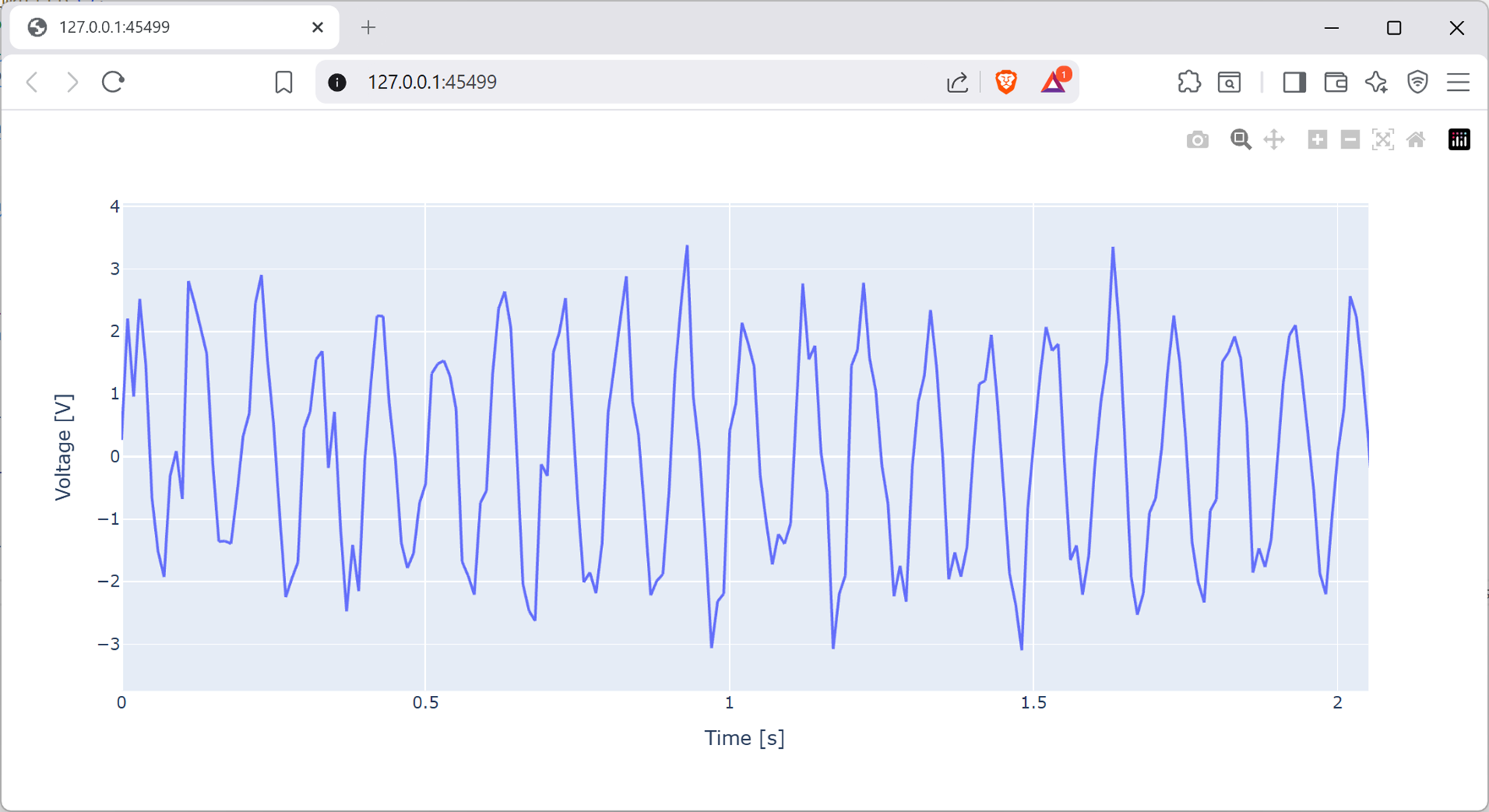
Screenshot of a web browser, software from Brave. See course copyright statement.¶

This is a 10 Hz sine wave, corrupted by some high frequency noise. It’s the same as the signal we made the first part of the lab by adding random noise to a 10 Hz sine wave, we’ve now just loaded it in from a file.

Scipy contains functions for filtering this noise out. Add the function below to your code, edit the rest of the code to call this function, and plot the filtered signal. You’ll need to work out the correct parameters to pass to filter_data().

def generate_filter_coefficients(cutoff, fs, order, ftype):
    """Calculate filter coefficients for a Butterworth filter"""
    nyq = 0.5 * fs  # expects the cutoff frequency to be given in Hz, it then scales this to be in the range 0 to 1, where 1 is half the sampling frequency
    normalized_cutoff = cutoff / nyq
    b, a = signal.butter(order, normalized_cutoff, btype=ftype, analog=False)
    return b, a


def filter_data(data, cutoff, fs, order, ftype):
    """Filter the data"""
    b, a = generate_filter_coefficients(cutoff, fs, order, ftype)
    signal_filtered = signal.filtfilt(b, a, data)
    return signal_filtered

This is implementing a Butterworth filter, which you will have learnt about in your electronics courses. It attenuates frequencies higher than the cutoff.

Solution

if __name__ == "__main__":
    t, v = load_signal_from_matfile()
    fs = 1 / (t[1] - t[0])
    v_filtered = filter_data(v, 50, fs, 1, "low")
    px.line(
        x=t[0:1000], y=v_filtered[0:1000], labels={"x": "Time [s]", "y": "Voltage [V]"}
    ).show()

Here the cut-off is set to be 50 Hz. The filtered signal will look like the below.

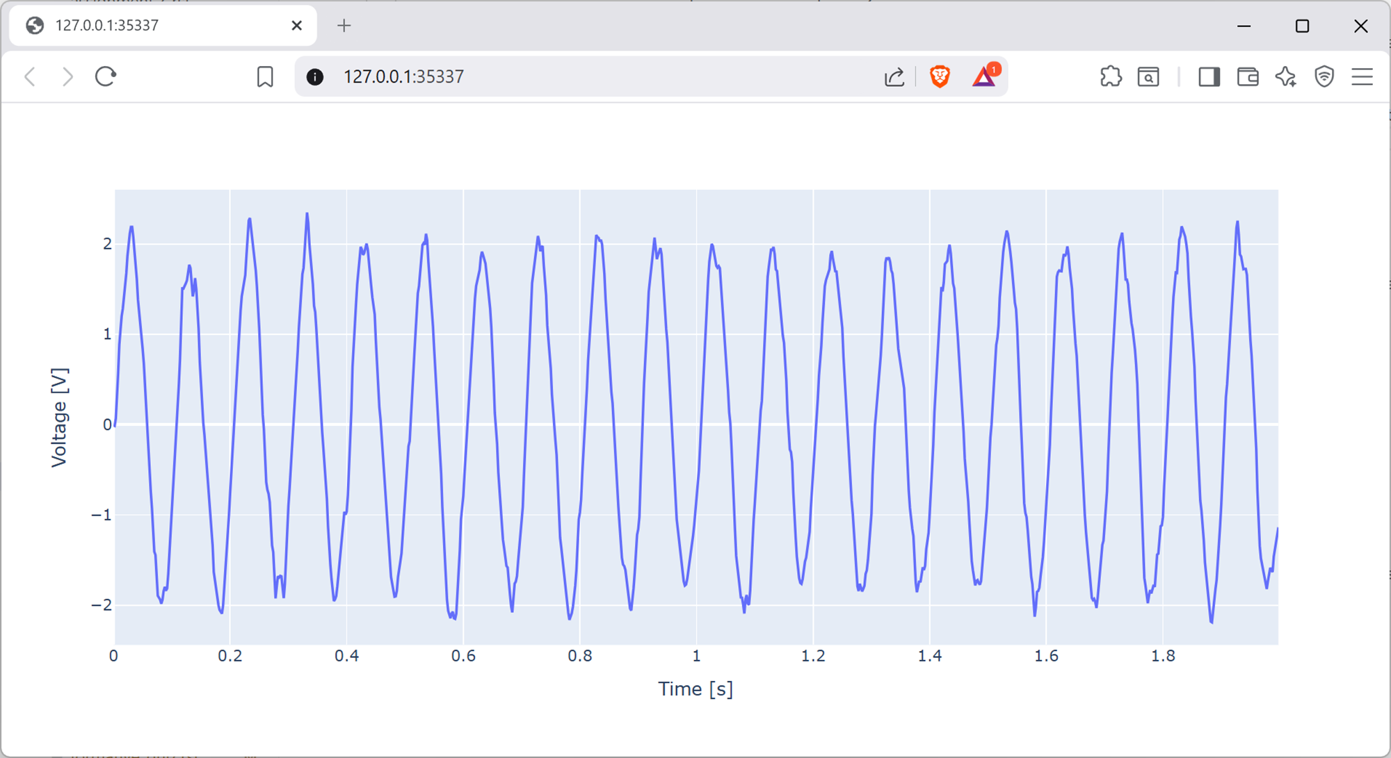
A filtered sine wave plotted with plotly — Screenshot of a web browser, software from Brave. See course copyright statement.¶

Assuming you’ve implemented the filtering as in the solution above, the sine wave still looks quite noisy. By using different filtering functions as given in the scipy signal documentation, or otherwise, try and clean the signal more to make it look like a pure sine wave.

Solution

The simplest approach will just be to change the order of the filter, and the cut-off. Our example code uses a first order filter with a cut-off of 50 Hz. We know the sine wave is at 10 Hz, so the cut-off can probably be a bit lower. First order is quite low for a filter. Taking the order too high will introduce a different type of distortion (covered in your filters courses), but it can probably be second or fourth order without issue.

There are also lots of different filtering functions in scipy that you can try here, and we’ll leave you to experiment.

4.2.2.2. Signal detection example¶

Your Lab E data folder also contains a file called ecg.mat, which contains vectors time and ecg. Write a Python script that loads and plots this data. The start of the plot will look like the below.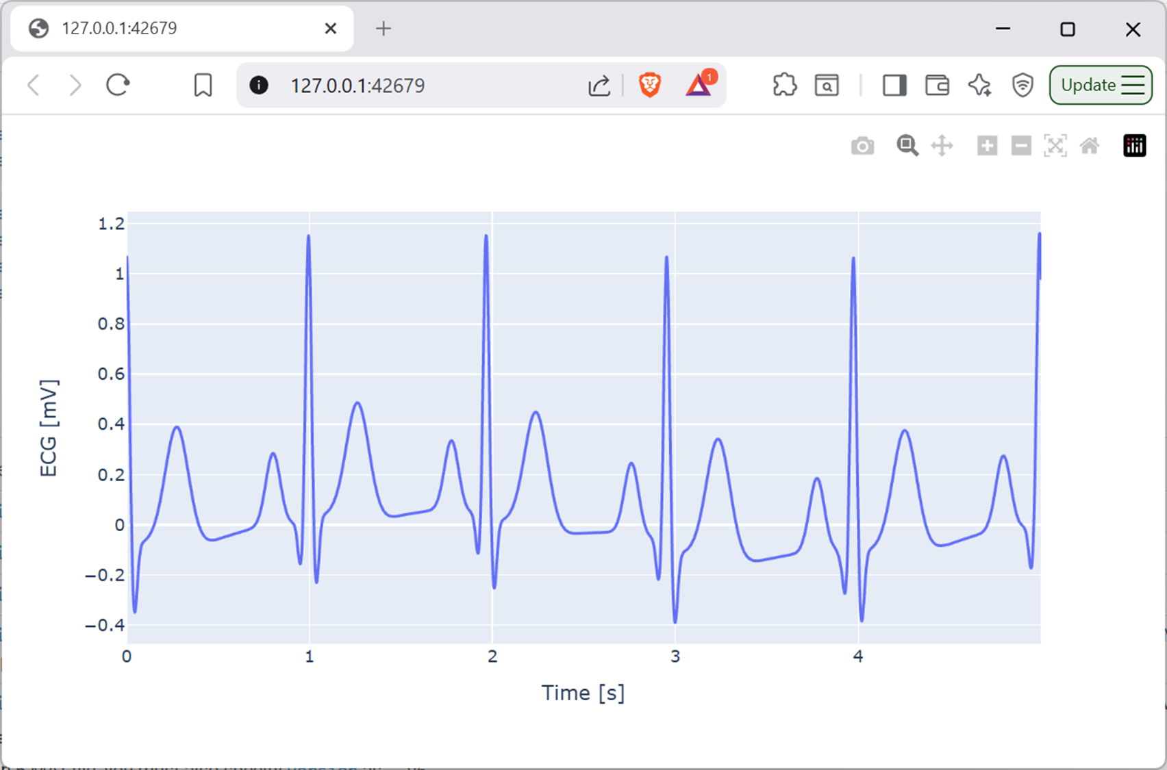

An ECG trace plotted with plotly — Screenshot of a web browser, software from Brave. See course copyright statement.¶

Solution

import pathlib
from os.path import join as pjoin

import numpy as np
import plotly.express as px
import scipy.io as sio


def load_signal_from_matfile():
    # Get the path to the .mat file
    # This uses pathlib to automatically get the folder where this script is located and navigates from there
    script_folder = pathlib.Path(__file__).parent.resolve()
    data_dir = pjoin(script_folder, "../", "data")
    mat_fname = pjoin(data_dir, "ecg.mat")

    # Load data
    data = sio.loadmat(mat_fname, variable_names=["time", "ecg"])
    return data["time"].squeeze(), data["ecg"].squeeze()


if __name__ == "__main__":
    time, ecg = load_signal_from_matfile()
    fs = 1 / (time[1] - time[0])
    plot_duration = 5  # seconds
    px.line(
        x=time[0 : int(fs * plot_duration)],
        y=ecg[0 : int(fs * plot_duration)],
        labels={"x": "Time [s]", "y": "ECG [mV]"},
    ).show()

Aside

This is an electrocardiography (ECG) signal. It represents the electrical activity of the heart. Many smartwatches now include ECG monitors as part of their health and wellbeing features. Clinically, the ECG is regularly used to diagnose a wide number of heart related conditions.

The example in our labs is simulated, using the code from ecgsyn, but there are many real ECG recordings on PhysioNet that you can explore if you’re interested.

Scipy also includes an example ECG dataset that you can load directly using scipy.misc.electrocardiogram().

In the ECG signal there are some clear, sharp, peaks. These correspond to heart beats. Write code to automatically detect these peaks using the signal.find_peaks() function. As such, calculate the average heart rate in beats per minute (bpm) over the duration of the recording.

Hint

You’ll find that too many peaks are detected using the default settings for signal.find_peaks(). To get a good estimation you’ll need to change the settings for how a peak is detected. See the documentation for signal.find_peaks() here to see the options available.

You might find it helpful to plot the detected peaks on top of the ECG signal to see which points have been detected. This requires plotting two lines on the same graph, which we’ll cover in Lab F if you want to skip ahead.

Solution

The average heart rate for this record is 60 beats per minute (bpm).

import pathlib
from os.path import join as pjoin

import numpy as np
import plotly.express as px
import scipy.io as sio
from scipy import signal


def load_signal_from_matfile():
    # Get the path to the .mat file
    # This uses pathlib to automatically get the folder where this script is located and navigates from there
    script_folder = pathlib.Path(__file__).parent.resolve()
    data_dir = pjoin(script_folder, "../", "data")
    mat_fname = pjoin(data_dir, "ecg.mat")

    # Load data
    data = sio.loadmat(mat_fname, variable_names=["time", "ecg"])
    return data["time"].squeeze(), data["ecg"].squeeze()


if __name__ == "__main__":
    # Load data
    time, ecg = load_signal_from_matfile()
    fs = 1 / (time[1] - time[0])

    # Detect peaks
    peaks, _ = signal.find_peaks(
        ecg,
        height=0.5,  # minimum height of peaks - will work for this record, but don't be very robust for different traces with differnt amplitudes
    )  # _ indicates we ignore the second output from find_peaksS

    # Calculate heart rate
    duration = time[-1]  # total duration in seconds is the last value in time
    num_beats = len(peaks) / duration  # average beats per second
    bpm = num_beats * 60  # convert to beats per minute
    print(f"Average heart rate: {bpm:.1f} bpm")

    # Do plots
    plot_duration = 5  # seconds
    fig = px.line(
        x=time[0 : int(fs * plot_duration)],
        y=ecg[0 : int(fs * plot_duration)],
        labels={"x": "Time [s]", "y": "ECG [mV]"},
    )
    fig.add_scatter(
        x=time[peaks[peaks < fs * plot_duration]],
        y=ecg[peaks[peaks < fs * plot_duration]],
        mode="markers",
        marker=dict(color="red", size=8),
        name="Detected Peaks",
    )
    fig.show()

Check your code in to Git before proceeding.

4.2.2.3. Further (optional) tasks¶

Usually we don’t want to estimate the heart rate from the entire signal. This would mean waiting a long time to get all of the data.

It’s common (in wearables) that we estimate heart rate using 8 second windows of data. Every 2 s this window moves on, so there’s 6 seconds of overlap between each window. This means that every 2 s we get a new estimate of heart rate, based on the last 8 seconds of data. We can then get a plot of heart rate over time.

Within each window of data we calculate the heart rate with the equation

\[hr = 60 \times \frac{n_{beats} - 1 }{t_{last} - t_{first}}\]

where \(n_{beats}\) is the number of detected beats in the window, and \(t_{last}\) and \(t_{first}\) are the times of the last and first detected beats in the window respectively.

Write code to implement this sliding window heart rate estimation, and plot the resulting heart rate over time.

Solution

import pathlib
from os.path import join as pjoin

import numpy as np
import plotly.express as px
import scipy.io as sio
from scipy import signal


def load_signal_from_matfile():
    # Get the path to the .mat file
    # This uses pathlib to automatically get the folder where this script is located and navigates from there
    script_folder = pathlib.Path(__file__).parent.resolve()
    data_dir = pjoin(script_folder, "../", "data")
    mat_fname = pjoin(data_dir, "ecg.mat")

    # Load data
    data = sio.loadmat(mat_fname, variable_names=["time", "ecg"])
    return data["time"].squeeze(), data["ecg"].squeeze()


def detect_ecg_peaks(ecg):
    peaks, _ = signal.find_peaks(
        ecg,
        height=0.5,  # minimum height of peaks - will work for this record, but don't be very robust for different traces with differnt amplitudes
    )  # _ indicates we ignore the second output from find_peaks
    return peaks


def process_ecg_window(time, ecg, fs):
    # Calculate number of windows
    window_size = 8  # seconds
    step = 2  # seconds
    num_windows = int((time[-1] - window_size) // step) + 1

    # Preallocate heart rate array
    hr = np.zeros(num_windows)
    time_hr = np.zeros(num_windows)

    # Process each window of data in turn
    for w in range(num_windows):
        # Get window of data
        start_idx = int(w * step * fs)
        end_idx = int(start_idx + window_size * fs)
        ecg_window = ecg[start_idx:end_idx]
        time_window = time[start_idx:end_idx]

        # Detect peaks in the window
        peaks = detect_ecg_peaks(ecg_window)

        # Calculate heart rate for the window
        hr[w] = 60 * (len(peaks) - 1) / (time_window[peaks[-1]] - time_window[peaks[0]])
        time_hr[w] = time_window[-1] + 1 / fs

    return time_hr, hr


if __name__ == "__main__":
    # Load data
    time, ecg = load_signal_from_matfile()
    fs = 1 / (time[1] - time[0])

    # Detect peaks
    time_hr, hr = process_ecg_window(time, ecg, fs)

    # Plot heart rate
    fig = px.line(
        x=time_hr,
        y=hr,
        labels={"x": "Time [s]", "y": "Heart Rate [bpm]"},
        line_shape="hv",
    ).show()

In ecg.mat there is another variable called ecg_noise, which is a noisier version of the ECG signal. Try and detect the peaks in this noisier signal. You might need to do some filtering first to clean up the signal before peak detection will work well, and/or make your peak detection function more robust.

Solution

We don’t have example code for this task, it’s one for you to try and experiment with. The underlying ECG signal is exactly the same as in the earlier example, just with more noise, so you can compare your estimates from the two signals to see how well you’re doing.