6.2.1. Writing code for AI¶

6.2.1.1. Initial setup for the Lab¶

In the VSCode terminal enter:
```
cd /workspaces/`ls /workspaces`/lab-i
uv init .
```
Remember to enter these one at a time, not both together.

This will make a new Python project in the current folder. It will be named automatically after the folder name.

To analyze these lines:
- cd /workspaces/`ls /workspaces`/lab-i makes sure we are working in the lab-i folder.
- uv init . is the interesting command. This actually sets up our virtual environment.
The above will make the a pyproject.toml file, a main.py file, and a number of others.
Add some structure to your folder by entering the commands:
```
mkdir tests docs
mv main.py src
uv run src/main.py
touch tests/__init__.py
```
- Here we’ve moved main.py into the src folder. You’ll see that the src folder contains some code that we’ve written for you.
- We’ve made a tests folder for any tests that we might want to write later, and a docs folder for any documentation.
- In the files that were downloaded from Git automatically, you’ll also see there’s a folder called data. This contains some files that we’ll analyze during the lab.

Install the required dependencies for this lab by entering the command:

uv add torch torchvision torchmetrics scipy plotly pandas nbformat

Run
```
uv run src/main.py
```
to make sure the virtual environment is built.
When you open a Python file, make sure that the correct Python virtual environment is activated. See the instructions in Lab D if you’re unsure.

6.2.1.2. Overview¶

Python is very widely used for writing code for AI models. Commands for AI are not part of the standard library, they are added in as external modules. PyTorch and TensorFlow are two of the most widely used libraries for AI coding in Python. Here we will use PyTorch.

This is not a course about AI, but there are a few basics that you’ll need to know in order to follow along. There are several steps in writing code for AI models. These are:

We need a problem statement. That is, we need to know what we want the AI to do.
We need data that the AI can use to tackle the problem statement. E.g. if we want to automatically tell the colour of a car, we’ll need some pictures of cars, ideally labelled with their colours.
The data is usually split into three parts training, validation, and testing. Training data is used to make the model in the first place, it gives the AI data that it can learn from. Validation data is used to check the training. The training will be repeated if the validation performance isn’t good enough. Testing data is used to see how well the model works, by giving it data that it hasn’t seen before.
We often need to do some pre-processing of the data before passing it to the AI. This might include cleaning the data (e.g. removing missing or invalid entries), normalizing the data (e.g. making sure all values are on a similar scale), or selecting key points (features) so that these are used as the input for the AI rather than all of the raw data. This step might be known as transforming the data, or carrying out feature generation and feature selection. There might be some other factors to take into account, such as making sure that the data is well shuffled so that the training works well, deciding on a batch size (how many data points are used in each step of the training), and so on, which we won’t look into here.
We then decide on a model architecture. There are lots of different types of AI, with different advantages and disadvantages for different problem statements and types of data. Often the same architecture has a wide range of choices or parameters that can be adjusted.
We train the model.
We test the model and obtain some performance metrics for how well it did.
When we’re happy, we can deploy the model. That is, actually use it in practice.

Note

We won’t cover model deployment here.

We also won’t make a separate validation data set, to make the examples a bit more compact. You almost certainly do want a validation data set if you’re working on a real problem.

A full copy of the code for this lab is given in your Lab I src folder as solution.py which you can refer to if you’re not sure where any individual piece of code should go.

6.2.1.3. Problem statement¶

We’re going to look at a classification problem, which is a very common AI task. We have a database of pictures of flowers, and we want the AI to be able to tell us what type of flower is in a picture. We’ve picked this as an example because it will illustrate all of the key steps for us, and the data required is readily available and doesn’t use a lot of disc space.

Our problem is going to be supervised. This is, for training the network we have already collected some data where we know what the correct answer is. The AI can use this input and the answer, to learn the relationship between the two.

6.2.1.4. Data set¶

In practice when making AI you likely either:

Already have data that’s been collected for you and you have to work with (possibly regardless of whether it’s a very good fit for your problem statement). The data may be public data from the Internet, which is what we’ll use here.
Collect your own data, which may be expensive and time-consuming, but can mean you definitely get the data that you want.

To help people get started, there are a number of public data sets available online and PyTorch includes dedicated commands to download them. Here we’ll use a Flowers Recognition data set, which contains labelled pictures of flowers of different types. This dataset was made by: Nilsback, M-E. and Zisserman, A. in Automated flower classification over a large number of classes. Proceedings of the Indian Conference on Computer Vision, Graphics and Image Processing (2008). PyTorch contains built in functions to download and use widely used public datasets like this one. If you’re using your own data, it might be a bit more work to first load the data (say from a .mat file as we saw in Lab E), and then convert it into a format that PyTorch can use. We won’t cover this here.

Edit your src/main.py file and edit it to be the following:

import numpy as np
import plotly.express as px
import torch
from torch import nn
from torch.utils.data import DataLoader
from torchmetrics.classification import (
    MulticlassAccuracy,
    MulticlassConfusionMatrix,
)
from torchvision import datasets
from torchvision.transforms.v2 import Compose, Resize, ToDtype, ToImage


def get_data(data_folder, image_size, clean_run=True):
    # Get training data
    training_data = datasets.Flowers102(
        root=data_folder,
        split="train",
        download=clean_run,
        transform=Compose(
            [
                Resize((image_size, image_size)),
                ToImage(),
                ToDtype(torch.float32, scale=True),
            ]
        ),
    )

    # Get test data
    test_data = datasets.Flowers102(
        root=data_folder,
        split="test",
        download=clean_run,
        transform=Compose(
            [
                Resize((image_size, image_size)),
                ToImage(),
                ToDtype(torch.float32, scale=True),
            ]
        ),
    )


if __name__ == "__main__":
    # Settings
    data_folder = "data"  # put in data folder in project root
    image_size = 500  # images will be resized to 500x500

    # Run network steps
    training_data, test_data = get_data(data_folder, image_size, clean_run=True)

Run this code. It will download the data set into your Lab I data folder. It will likely take a few minutes and you may not see much output while it’s running. When it’s done, you should see that a number of files have been downloaded into the data folder.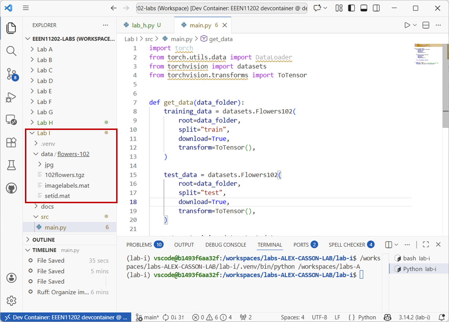

Screenshot of VSCode, software from Microsoft. See course copyright statement.¶

Open some of the files in the jpg folder and you should see some flowers.

The end result is training_data and test_data which are Dataset objects, dedicated objects for how PyTorch wants the data organized for working with.

Note that we gave the get_data() function an argument clean_run=True. If this is set to True, the data will be downloaded again each time you run the code. You probably don’t want this once you’ve downloaded the data. To save time you can switch this to False after the first run.
The get_data() function actually does several of the AI pipeline steps for us. We downloaded training and test datasets separately. The lines
```
transform=Compose(
    [
        Resize((image_size, image_size)),
        ToImage(),
        ToDtype(torch.float32, scale=True),
    ]
)
```
do the pre-processing for us.

If you look closely at the raw images you’ll see that they’re all slightly different sizes. Some have 500 pixels on one size, some 520, and so on. The PyTorch Resize command makes them all have the same number of pixels, as the AI needs a consistent input. Resize is a built in pre-processor in PyTorch for working with images. There are others, listed in the documentation. You can also define your own preprocessor by writing a custom class if you need to.

ToImage and ToDtype are built in transforms that we just need to make everything work in this example. PyTorch expects to work with numbers, and so we need to make sure Python is storing the image as numbers in the correct format, rather than as an image object.

The end result is train_data and test_data. You can see that we downloaded different data for the training and testing sets, so we don’t need to do anything more here. In practice, it can be quite a lot of work to decide how to best split data into training and test. For example, if you’re working with time series, you don’t want to have data from the future in your training set!

Spend some time exploring the dataset. For example, you can see the different classes (types of flower) with training_data.classes. You can see the label for training image number (say 42) with _, label = training_data[42]. Can you make a histogram of the number of images in each class?

Solution

def plot_training_label_histogram(data):
    label_list = [label for _, label in data]
    fig0 = px.histogram(label_list)
    fig0.update_layout(
        xaxis=dict(
            title="Flower label",
            tickmode="array",
            tickvals=list(range(0, len(data.classes))),
            ticktext=data.classes,
        ),
    )
    fig0.show()

In principle we could start using the above for the machine learning. In practice we nearly always arrange the data into batches first. A batch is a small group of data points that are used together in one step of the training. This is done putting the data into a DataLoader object. Add the following function to your src/main.py file, we literally just need to say what batch size we want to use with which piece of data.

...

def make_data_loaders(training_data, test_data):
    # Make data loaders
    batch_size = 128
    train_dataloader = DataLoader(training_data, batch_size=batch_size)
    test_dataloader = DataLoader(test_data, batch_size=1)

    return train_dataloader, test_dataloader

...

if __name__ == "__main__":
    # Settings
    data_folder = "data"  # put in data folder in project root
    image_size = 500  # images will be resized to 500x500

    # Run network steps
    training_data, test_data = get_data(data_folder, image_size, clean_run=False)
    plot_training_label_histogram(training_data)
    train_dataloader, test_dataloader = make_data_loaders(training_data, test_data)

6.2.1.5. Model architecture¶

There are lots of built in models in PyTorch that you can use directly, or you can use a pre-trained model and fine-tune it for your own data. For example, for this image classification problem you might use a pre-trained ResNet model. We will make a simple model by hand (which won’t actually get very good performance, but illustrates the key steps and is quick to train).

Add the function below to your src/main.py file, and call it in the if __name__ == "__main__": section after getting the data.

def make_model_architecture(image_size, num_classes):
    # Use GPU acceleration if available
    device = (
        torch.accelerator.current_accelerator().type
        if torch.accelerator.is_available()
        else "cpu"
    )

    # Define neural network model
    class NeuralNetwork(nn.Module):
        def __init__(self):
            super().__init__()
            self.flatten = nn.Flatten()
            self.linear_relu_stack = nn.Sequential(
                nn.Linear(
                    image_size * image_size * 3, 128
                ),  # image size times 3 color channels
                nn.ReLU(),
                nn.Linear(128, 128),
                nn.ReLU(),
                nn.Linear(128, num_classes),  # 102 flower classes
            )

        def forward(self, x):
            x = self.flatten(x)
            logits = self.linear_relu_stack(x)
            return logits

    model = NeuralNetwork().to(device)
    print(model)

return model, device

...

if __name__ == "__main__":
    # Settings
    data_folder = "data"  # put in data folder in project root
    image_size = 500  # images will be resized to 500x500

    # Run network steps
    training_data, test_data = get_data(data_folder, image_size, clean_run=False)
    plot_training_label_histogram(training_data)
    train_dataloader, test_dataloader = make_data_loaders(training_data, test_data)
    model, device = make_model_architecture(
        image_size, num_classes=len(training_data.classes)
    )

Fundamentally, a model is defined by a class, as we learnt about in Lab G. It has two methods. The __init__() method defines the AI model that we want. It is made up of a number of layers and the connections between these layers.The forward() method defines how data passes through the model.

As this isn’t a course on AI, and so we’ll just stick with these choices for the number of layers, the types of layers, values and so on, and move on. Of course these values are extremely important to the overall performance of the network, and will require some design and tuning to get them right for a real problem.

Run the code. You should see a summary of the model printed out like the below:

NeuralNetwork(
  (flatten): Flatten(start_dim=1, end_dim=-1)
  (linear_relu_stack): Sequential(
    (0): Linear(in_features=750000, out_features=128, bias=True)
    (1): ReLU()
    (2): Linear(in_features=128, out_features=128, bias=True)
    (3): ReLU()
    (4): Linear(in_features=128, out_features=102, bias=True)
  )
)

6.2.1.6. Training the model¶

As noted earlier, we don’t usually train a model all in one go, we split the data into batches. Our training is thus in a for loop. There are again many choices for how we do the training. We are carrying out supervised learning and so generally the network will try to generate an answer from an input, compare this to the known correct answer, and then adjust the model to try and reduce the number of times there is a difference between its answer and the correct answer. This is done using an optimizer and a loss function. We’re going to use CrossEntropyLoss as the loss function and SGD (Stochastic Gradient Descent) as the optimizer.

Add the function below to your src/main.py file, and call it in the if __name__ == "__main__": section after defining the model.

def train_model(model, train_dataloader, device):
    loss_fn = nn.CrossEntropyLoss()
    optimizer = torch.optim.SGD(model.parameters(), lr=1e-3)
    model.train()
    for batch, (X, y) in enumerate(train_dataloader):
        X, y = X.to(device), y.to(device)
        pred = model(X)
        loss = loss_fn(pred, y)
        loss.backward()
        optimizer.step()
        optimizer.zero_grad()

        # Print progress - generally want to see loss decreasing
        # We wouldn't usually print every batch, but this is a small dataset
        loss, loss.item()
        print(f"Batch: {batch}, loss: {loss:>7f}")

        print("Training complete.")
        return model

...

if __name__ == "__main__":
    # Settings
    data_folder = "data"  # put in data folder in project root
    image_size = 500  # images will be resized to 500x500

    # Run network steps
    training_data, test_data = get_data(data_folder, image_size, clean_run=False)
    plot_training_label_histogram(training_data)
    train_dataloader, test_dataloader = make_data_loaders(training_data, test_data)
    model, device = make_model_architecture(
        image_size, num_classes=len(training_data.classes)
    )
    train_model(model, train_dataloader, device)

6.2.1.7. Testing the model¶

Testing the model is in many ways similar to how we train the model. We again use a for loop to go through the test data in batches. As this is a supervised problem, we can compare the model’s output (known as a prediction) to the true label or target for the data file being analyzed. We can then generate stats to summarize how well the model did. There are built in functions for doing this. We’re going to use MulticlassAccuracy to get the overall accuracy, and MulticlassConfusionMatrix to get a confusion matrix, which is a more visual illustration.

Add the function below to your src/main.py file, and call it in the if __name__ == "__main__": section after defining the model.

def test_model(model, test_dataloader, classes, device):
    model.eval()

    # Go through each image in the test set in turn, pass it to the model with model(image)
    out = []  # used for generating the confusion matrix later
    for batch, (X, y) in enumerate(test_dataloader):
        with torch.no_grad():
            X = X.to(device)
            pred = model(X)
            pred_output = pred[0].argmax(0)
            predicted, actual = (
                classes[pred_output],
                classes[y],
            )
            print(f"Image no.: {batch} Predicted: {predicted}, Actual: {actual}")
            out.append((int(pred_output), int(y)))

    # Combine all predictions and actual labels into tensors for calculating overall metrics on
    y_true = torch.tensor([x[1] for x in out])
    y_pred = torch.tensor([x[0] for x in out])

    # Generate confusion matrix
    metric = MulticlassConfusionMatrix(num_classes=len(classes))
    print(metric(y_pred, y_true))

    # Calculate overall accuracy
    metric = MulticlassAccuracy(num_classes=len(classes))
    acc = metric(y_pred, y_true)  # overall accuracy
    print(f"Accuracy over test set: {acc:.4f}")
    metric = MulticlassAccuracy(num_classes=len(classes), average=None)
    per_class_acc = metric(y_pred, y_true)  # per-class accuracy
    print(f"Per-class accuracy: {per_class_acc}")

...

if __name__ == "__main__":
    # Settings
    data_folder = "data"  # put in data folder in project root
    image_size = 500  # images will be resized to 500x500

    # Run network steps
    training_data, test_data = get_data(data_folder, image_size, clean_run=False)
    plot_training_label_histogram(training_data)
    train_dataloader, test_dataloader = make_data_loaders(training_data, test_data)
    model, device = make_model_architecture(
        image_size, num_classes=len(training_data.classes)
    )
    train_model(model, train_dataloader, device)
    test_model(model, test_dataloader, test_data.classes, device)

Run the code. Your final output should look similar to the below.

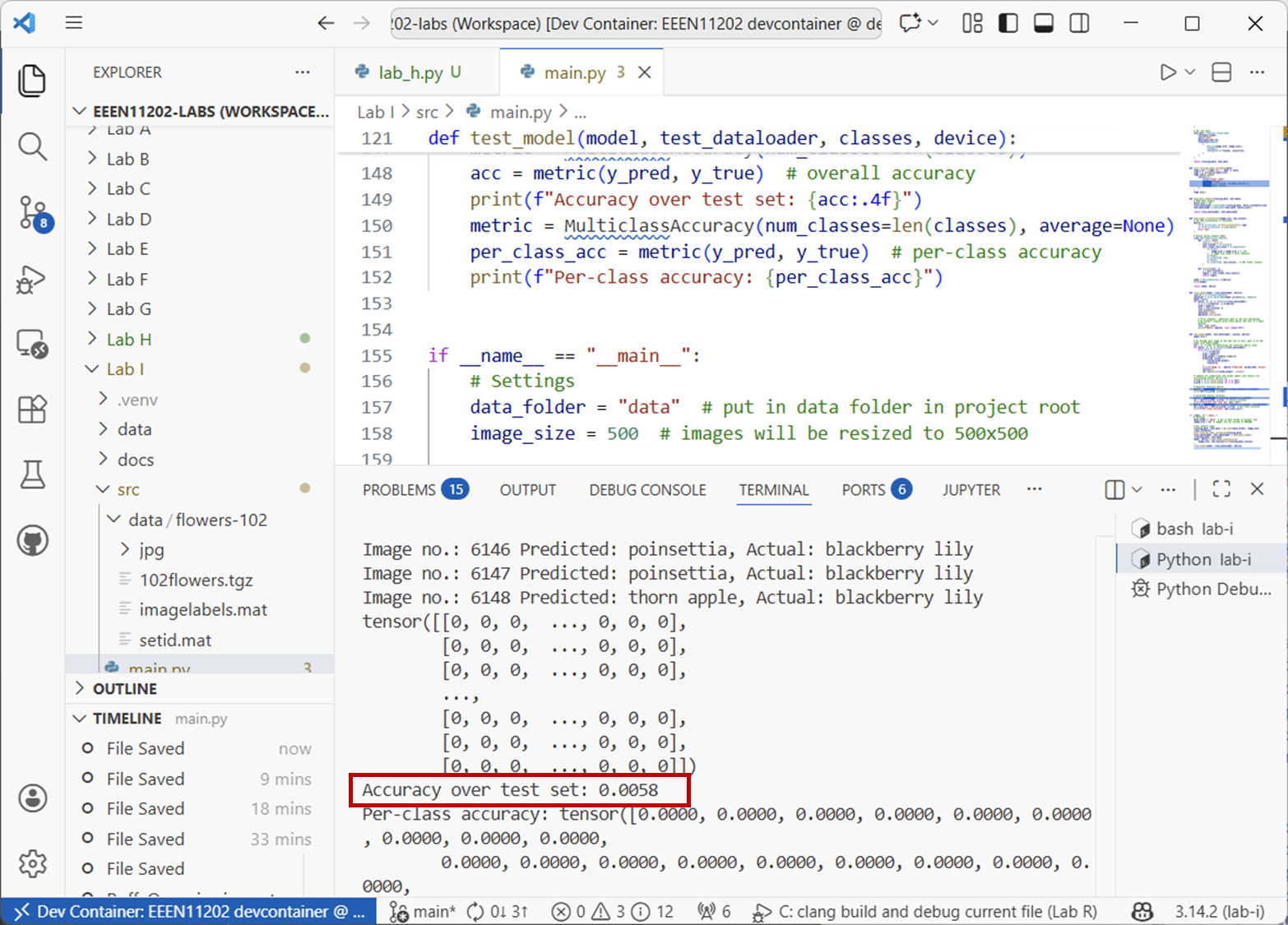
Screenshot of VSCode, software from Microsoft. See course copyright statement.¶

The overall accuracy (in this screenshot) is 0.6%.
You might notice two things. Firstly, if you run the code again, you’ll get a slightly different output. To start the training, the model parameters are usually randomly initialized. Each time you run the code you’ll get different random numbers as the starting point. In practice you might want to set a fixed random seed so that you can get repeatable results.

Secondly, this is accuracy is very low! Indeed, there are things we can do to check, but it’s probably chance level. We have 102 classes in this problem, and a roughly equal number of examples of each class. Thus, if we just used a random number generator we’d expect it to pick the right class 1/102 of the time on average, which is about 0.98%. If you look closely at the output, you’ll see that nearly everything is being put into the same class, it thinks it is the same type of flower every time. This is quite common with simple small networks like this, it hasn’t actually learnt anything useful yet.

6.2.1.8. Making the network better¶

Fundamentally, we’ve been through all of the different steps needed for AI in Python using PyTorch. For most practical problems, you will just need to spend much more time on each one of the steps. For example, processing the data, normalizing the data, deciding on the model architecture, tuning the model hyperparameters, and so on. We don’t know what computers students are using, and so we deliberately kept the model small so that it would run in a reasonable amount of time on most machines. The negative of this is that it gets very poor performance.
We’ll leave it as an open ended problem for you to explore for how to get better performance. It shouldn’t be too hard to get accuracies of 90% or more for this dataset, with some effort. (Again we’ll leave you to decide how long you want to spend on this. There are no marks for it.) If you get particularly good performance, come and show us in the lab and maybe we’ll make your code an example for next year. Two things you might explore are:
- Using a pre-trained model such as ResNet rather than making your own from scratch. With this, you wouldn’t necessarily need to do your own training step. Information for this is online.
- Using a Convolutional Neural Network (CNN) architecture rather than a simple feed-forward network. CNNs are very widely used for image data. There are built in layers for CNNs in PyTorch, see here for more information.