4.3.1. Plotting with plotly and matplotlib
4.3.1.1. Initial setup for the Lab
In the VSCode terminal enter:
cd /workspaces/`ls /workspaces`/lab-f uv init .
Remember to enter these one at a time, not both together.
This will make a new Python project in the current folder. It will be named automatically after the folder name.
To analyze these lines:
cd /workspaces/`ls /workspaces`/lab-fmakes sure we are working in the lab-f folder.uv init .is the interesting command. It makes a simple pyproject.toml file to define the project. (The actual virtual environment is made automatically when we run code.)
The above will make the a
pyproject.tomlfile, amain.pyfile, and a number of others.Add some structure to your folder by entering the commands:
mkdir tests docs
mv main.py src
uv run src/main.py
touch tests/__init__.py
Here we’ve moved
main.pyinto thesrcfolder. You’ll see that thesrcfolder contains some code that we’ve written for you.We’ve made a
testsfolder for any tests that we might want to write later, and adocsfolder for any documentation. We won’t ask you to put anything into these as part of the lab instructions, but you might want to write some tests for your code to check that it’s working!In the files that were downloaded from Git automatically, you’ll also see there’s a folder called
data. This contains some files that we’ll analyze during the lab.
Install the required dependencies for this lab by entering the command:
uv add numpy scipy polars pandas matplotlib seaborn plotly fastexcel pyarrow nbformat ipykernel==6.31.0Run
uv run src/main.pyto make sure the virtual environment is built.
When you open a Python file, make sure that the correct Python virtual environment is activated. See the instructions in Lab D if you’re unsure.
4.3.1.2. Plotting examples
If there’s one thing that AI is good at, it’s helping to generate code for plotting data, remembering all of the different options that might be used to customize the display. As such, we’re not going to spend too long exploring lots of options. You’ll naturally pick up different ones as you use plotting libraries more often, and you can readily refer to documentation and AI tools to help with the details. Here we’ll look at a few examples to build some familiarity.
For this we’ll use the code:
import numpy as np


def make_example_signal(A, tau):
    """
    Make an example signal that rises exponentially
    Returns: t: time samples
    v: voltage samples
    """
    fs = 100  # sampling frequency in Hz
    t = np.arange(0, 1, 1 / fs)
    v = A * (1 - np.exp(-t / tau))
    return t, v


def get_student_marks():
    ''' Some example student marks for two courses '''
    marks_course_1 = np.array([
        81.0, 47.5, 76.1, 77.1, 84.5, 77.0, 67.2, 55.0, 99.0, 84.5,
        77.3, 72.4, 69.2, 66.2, 58.4, 58.5, 61.6, 66.0, 55.1, 61.5,
        81.0, 38.6, 68.9, 51.7, 62.7, 26.3, 86.0, 78.1, 81.1, 34.7,
        50.6, 69.0, 43.0, 52.3, 49.9, 29.1, 08.1, 93.1, 92.1, 55.2,
        56.1, 45.2, 49.6, 87.8, 65.0, 85.6, 40.4, 58.9, 89.6, 59.8,
        75.4, 62.6, 81.1, 58.9, 73.7, 56.8, 77.6, 53.5, 38.2, 56.5,
        80.5, 78.1, 73.6, 73.6, 67.8, 60.4, 81.2, 61.2, 70.0, 35.1,
        65.5, 85.6, 65.5, 26.9, 75.6, 65.1, 54.4, 72.9, 44.9, 92.9,
        49.2, 59.2, 45.6, 32.5, 89.5, 57.4, 73.2, 80.9, 68.1, 71.8,
        54.2, 55.0, 69.8, 31.1, 70.7, 81.1, 74.1, 48.2, 65.7, 80.4,
    ])

    marks_course_2 = np.array([
        15.3, 45.2,100.0, 57.9, 71.7, 93.4, 38.4, 86.4, 43.3, 52.2,
        56.8, 82.5, 51.8, 52.8, 76.2, 08.1, 70.3, 25.5, 27.1, 83.8,
        49.6, 52.5, 27.7, 82.9, 42.3, 62.7, 63.8, 83.0, 37.4, 51.0,
        20.9, 21.8, 68.8, 95.1, 76.5, 27.6, 61.5, 53.0, 04.3, 100.0,
        100.0,20.5, 00.0, 31.6, 12.6, 48.1, 44.0, 11.6, 45.1, 12.1,
        82.9, 48.7, 73.7, 35.2, 58.7, 32.7, 09.7, 32.1, 52.0, 69.0,
        72.2, 91.4, 72.3, 57.6, 41.0, 82.6, 43.5, 40.2, 11.6, 32.9,
        41.0, 76.6, 74.6, 49.9, 60.7, 29.0, 48.3, 58.8, 46.0, 40.4,
        49.0, 02.5, 77.6, 86.8, 75.3, 00.0, 89.0, 75.9, 60.3, 90.2,
        88.8, 03.0, 38.0, 43.0, 59.3, 30.8, 96.0, 42.5, 57.8, 74.9,
    ])

    return marks_course_1, marks_course_2


if __name__ == "__main__":
    # put code here
Setup
Make a new Python file in your Lab F
srcfolder calledplotly_examples.pyor similar. Copy the code given above into this.We’ve already added plotly as a dependency in the virtual environment, so in the code we only need to add the relevant import statements at the top of the file. To your code add
import plotly.express as px
import plotly.graph_objects as go
from plotly.subplots import make_subplots
We’re going to refer to plotly functions via the name
px.Run your code to check that there are no errors before proceeding. It won’t produce any outputs yet.
Notes
Before we get started, a few notes:
Plotly works very well with dataframes, which we’ll cover in the second part of the lab. We thus won’t use them here, but you’ll find that many online examples using Plotly just ask it to plot different columns in a dataframe. Plotly can then pick up the column heading (for example) for the legend automatically.
Below we’re using Plotly Express, abbreviated to
px, which provides a simple syntax for creating plots. To get more control over a figure you can use a graph object usingimport plotly.graph_objects as go. We won’t cover these here, apart from very briefly at the end when we look at subplots. More information is in the documentation at Plotly Graph Objects if you need to make more complicated plots. The general advice would be to make a basic plot using Plotly Express first, as we do below, and then if you need more control modify it using graph objects.We also won’t look at saving plotly plots to files here. We’ll cover that only for matplotlib. This reflects our approach of using plotly for interactive exploration of data, and matplotlib for making publication quality figures. If saving your plotly figures for a report or presentation, remember that you might want to adjust the font sizes and the resolution of the saved figure to make sure they look good.
Line plots
For electronic engineering, we’re often working with signals that vary over time, and so we plot these as a line so they look like traces on an oscilloscope. Add the code below to your Python file
if __name__ == "__main__":
    t, v = make_example_signal(A=5, tau=0.2)
    fig0 = px.line(x=t, y=v, labels={"x": "Time [s]", "y": "Voltage [V]"})
    fig0.show()
You’ll get a plot that shows a curve, similar to a capacitor charging up.
The basic syntax is fairly straightforwards. You need to explicitly call
.show()to display the plot. (This let you build up more complicated plots, and only display them when you’re ready.)The plot controls are hidden by default, but if you move the mouse to the top right of the plot, a number of controls will appear.
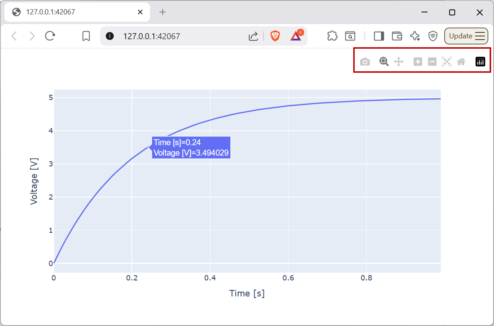
Screenshot of a web browser, software from Brave. See course copyright statement.
Try zooming in on the plot to see more detail. You can also hover over the line to see the exact values at each point. When you’re done, press the home button (the house icon) to return to the original view.
To add a second line, you use the
fig0object, and calladd_scatter(). This adds the data points, and we’ll set the mode tolinesso that it draws a line between the points.Remember to call
fig0.show()to actually draw the updated plot. We also have to add a legend for the first line that we had.# Add legend for first line fig0.data[0].showlegend = True fig0.data[0].name = "tau = 0.2 s" # Add second line with different tau t1, v1 = make_example_signal(A=5, tau=0.1) fig0.add_scatter( x=t1, y=v1, mode="lines", line=dict(dash="dot"), name="tau = 0.1 s" ) fig0.show()
Your figure should look like the below.
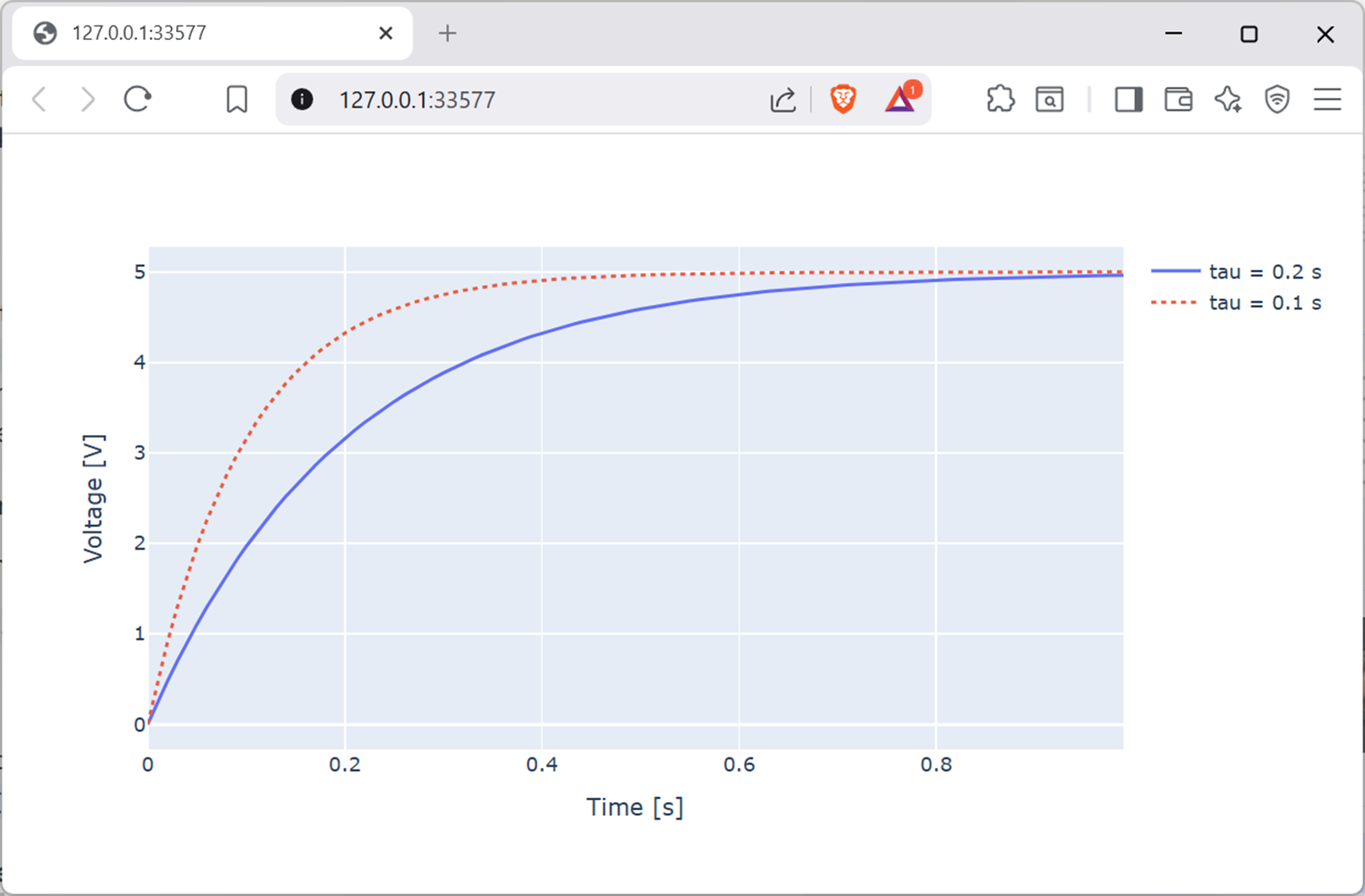
Screenshot of a web browser, software from Brave. See course copyright statement.
By searching the Internet, asking AI, or similar, modify your plot to change the line style and markers so that it looks like the below.
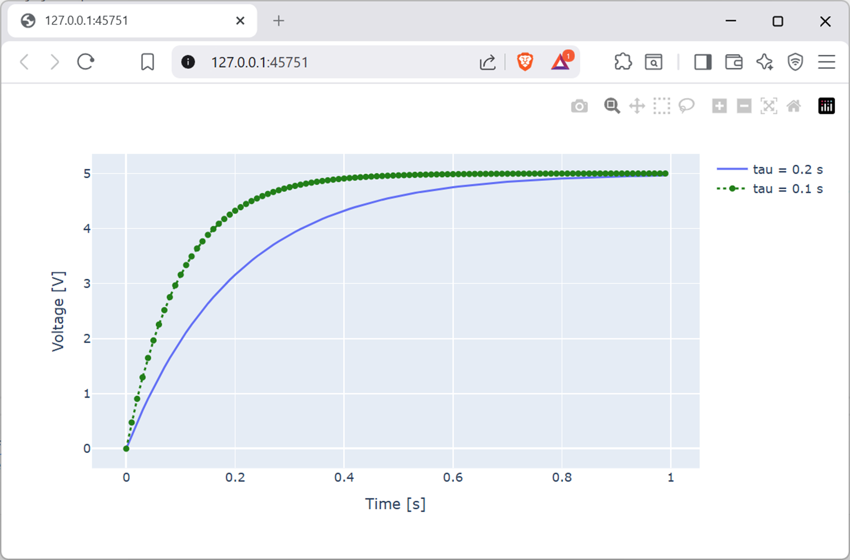
Screenshot of a web browser, software from Brave. See course copyright statement.
Solution
In this plot, the second line is green, and uses circle symbols to mark each data point. The code below modifies the existing line to change its style.
# Change the line style
# data[1] as we want the second line and we start counting from 0
# Could also look at fig0.update_traces()
fig0.data[1].line.color = "green"
fig0.data[1].marker.symbol = "circle"
fig0.data[1].mode = "lines+markers"  # show both lines and markers
fig0.show()
By searching the Internet, asking AI, or similar, add a vertical line at the time constant of each line (0.2 s and 0.1 s). You can do this using
.add_vline().Solution
 # Add vertical lines at the time constants
 fig0.add_vline(
    x=0.2,
    line=dict(color="blue", dash="dash"),
    annotation_text="0.2 s",
    annotation_position="top",
)
fig0.add_vline(
    x=0.1,
    line=dict(color="green", dash="dot"),
    annotation_text="0.1 s",
    annotation_position="top",
)
fig0.update_yaxes(
    range=[0, 5.2]
)  # line is drawn below 0 by default, so set y-axis range manually back to start at 0
fig0.show()
Other plot types
There are many different types of plot that you might want to make. Here are a few examples using the student marks data defined above.
Copy and paste the code below into your file to plot a histogram of the course 1 marks.
# Get student marks
marks_course_1, marks_course_2 = get_student_marks()

# Plot histogram of student marks
fig1 = px.histogram(
    marks_course_1,
    labels={"value": "Marks"},
)
fig1.update_layout(yaxis_title_text="Number of students")
fig1.show()
Copy and paste the below to make a box plot comparing the marks for course 1 and course 2. Which course did the students do generally better in?
# Make box plot comparing the two courses
fig2 = px.box(
    y=[marks_course_1, marks_course_2],
    labels={"variable": "Course"},
)
fig2.update_layout(
    yaxis_title_text="Marks",
    xaxis=dict(
        tickmode="array",
        tickvals=[0, 1],
        ticktext=["Course 1", "Course 2"],
    ),
)
fig2.show()
Solution
Course 1
Using
px.pie()make a pie chart like the below, showing the distribution of classifications in course 1.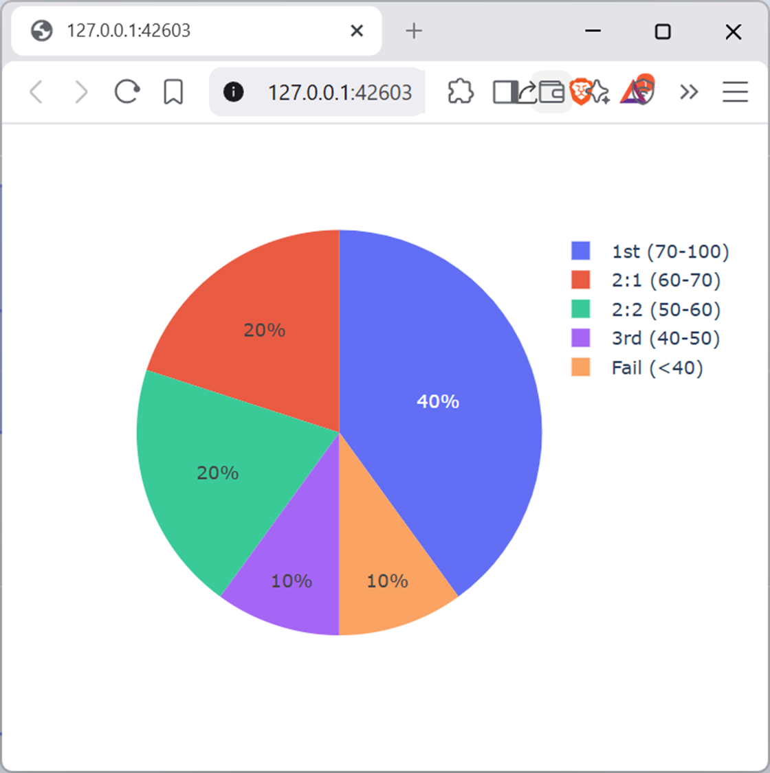
Screenshot of a web browser, software from Brave. See course copyright statement.
Solution
# Make a pie chart for grade distribution in course 1
boundaries = (100, 70, 60, 50, 40, 0)
fig3 = px.pie(
    names=[
        f"1st ({boundaries[1]}-{boundaries[0]})",
        f"2:1 ({boundaries[2]}-{boundaries[1]})",
        f"2:2 ({boundaries[3]}-{boundaries[2]})",
        f"3rd ({boundaries[4]}-{boundaries[3]})",
        f"Fail (<{boundaries[4]})",
    ],
    values=[
        np.sum(marks_course_1 >= boundaries[1]),
        np.sum(
            (marks_course_1 >= boundaries[2]) & (marks_course_1 < boundaries[1])
        ),
        np.sum(
            (marks_course_1 >= boundaries[3]) & (marks_course_1 < boundaries[2])
        ),
        np.sum(
            (marks_course_1 >= boundaries[4]) & (marks_course_1 < boundaries[3])
        ),
        np.sum(marks_course_1 < boundaries[4]),
    ],
)
fig3.show()
There are lots of plotly examples online. Try some of these out.
Subplots
Having more than one plot in a figure is often useful to compare different data.
If you add from plotly.subplots import make_subplots to your code, there is a function make_subplots() for building up subplots. There are two ways of doing this.
(The non-preferred method.) You can make a subplot, and then copy existing traces to this. Add the code below to your file and run it.
  fig = make_subplots(
      rows=2,
      cols=2,
      specs=[[{"type": "xy"}, {"type": "xy"}], [{"type": "xy"}, {"type": "domain"}]],
  )

  for trace in fig0.select_traces():
      fig.add_trace(trace, row=1, col=1)
  for trace in fig1.select_traces():
      fig.add_trace(trace, row=1, col=2)
  for trace in fig2.select_traces():
fig.add_trace(trace, row=2, col=1)
  for trace in fig3.select_traces():
      fig.add_trace(trace, row=2, col=2)
  fig.show()
You should get a plot like the below.
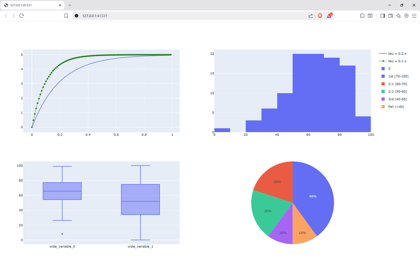
Screenshot of a web browser, software from Brave. See course copyright statement.
Here we’ve made a 2x2 grid of plots, and added the traces of each of the previous plots to one of the subplots. We haven’t copied the labels over, so these are missing at the moment.
Note that you need to tell plotly what type of plot each subplot is, using the
specsargument tomake_subplots()."xy"is for line plots, histograms, box plots, etc., while"domain"is for pie charts.(The preferred method.) You can make a subplot, and then use
.add_trace()to add data to each subplot directly. So far we’ve been using Plotly Expresspxto quickly build graphs. Unfortunately these aren’t compatible with.add_trace(). Instead we need to use Plotly Graph Objectsgoto give more control. We’re not going to cover them in a lot of detail here, but add the code below to your file as an example creating two Pie charts next to each other.fig5 = make_subplots( rows=1, cols=2, subplot_titles=("Course 1", "Course 2"), specs=[[{"type": "domain"}, {"type": "domain"}]], ) fig5.add_trace( go.Pie( labels=[ f"1st ({boundaries[1]}-{boundaries[0]})", f"2:1 ({boundaries[2]}-{boundaries[1]})", f"2:2 ({boundaries[3]}-{boundaries[2]})", f"3rd ({boundaries[4]}-{boundaries[3]})", f"Fail (<{boundaries[4]})", ], values=[ np.sum(marks_course_1 >= boundaries[1]), np.sum( (marks_course_1 >= boundaries[2]) & (marks_course_1 < boundaries[1]) ), np.sum( (marks_course_1 >= boundaries[3]) & (marks_course_1 < boundaries[2]) ), np.sum( (marks_course_1 >= boundaries[4]) & (marks_course_1 < boundaries[3]) ), np.sum(marks_course_1 < boundaries[4]), ], ), row=1, col=1, ) fig5.add_trace( go.Pie( labels=[ f"1st ({boundaries[1]}-{boundaries[0]})", f"2:1 ({boundaries[2]}-{boundaries[1]})", f"2:2 ({boundaries[3]}-{boundaries[2]})", f"3rd ({boundaries[4]}-{boundaries[3]})", f"Fail (<{boundaries[4]})", ], values=[ np.sum(marks_course_2 >= boundaries[1]), np.sum( (marks_course_2 >= boundaries[2]) & (marks_course_2 < boundaries[1]) ), np.sum( (marks_course_2 >= boundaries[3]) & (marks_course_2 < boundaries[2]) ), np.sum( (marks_course_2 >= boundaries[4]) & (marks_course_2 < boundaries[3]) ), np.sum(marks_course_2 < boundaries[4]), ], ), row=1, col=2, ) fig5.show()
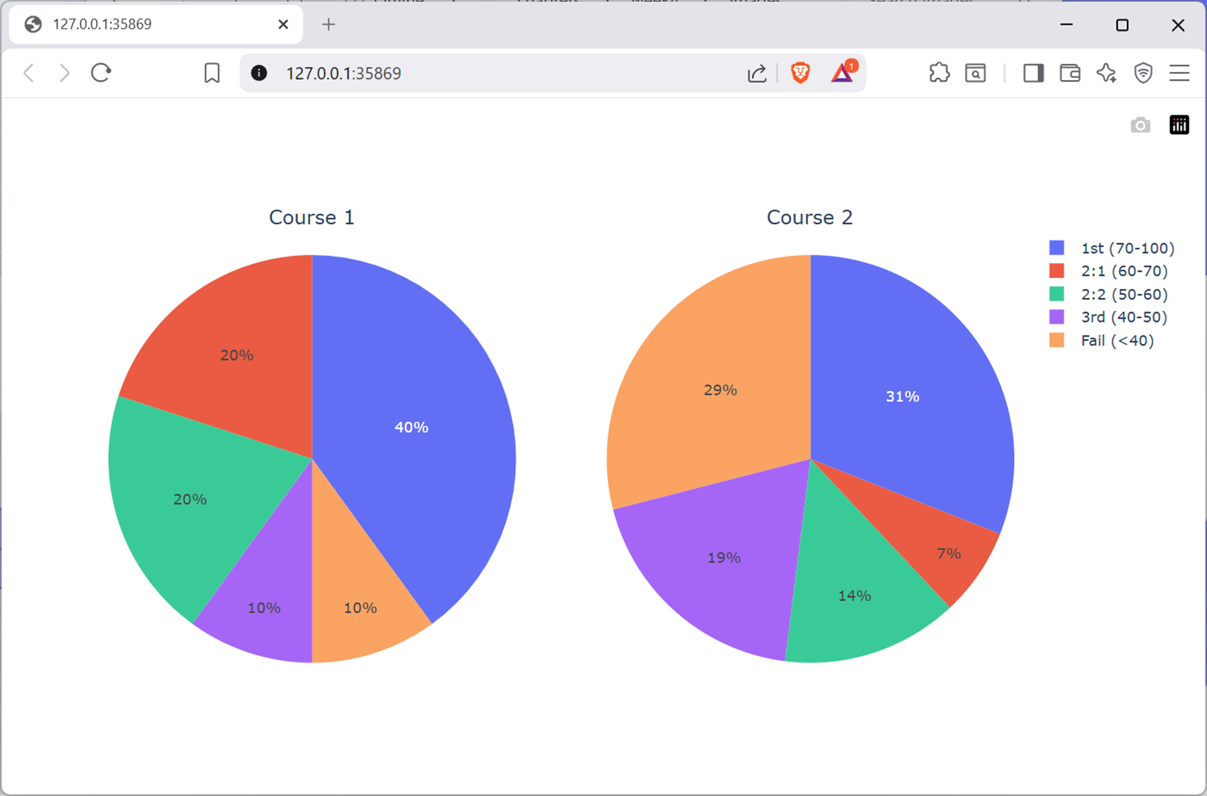
Screenshot of a web browser, software from Brave. See course copyright statement.
The plotting syntax using
gois very similar, but different to what we’ve used before. We won’t go into any more depth here, but this should give you enough of a starting point to build up your own plots to explore data.
Setup
Make a new Python file in your Lab F
srcfolder calledmatplotlib_examples.pyor similar. Copy the code given above into this.We’ve already added matplotlib and seaborn as dependencies in the virtual environment, so in the code we only need to add the relevant import statements at the top of the file. To your code add
import matplotlib.pyplot as plt
import numpy as np
import seaborn as sns
We’re going to refer to matplotlib functions via the name
plt.Then also add the code below to the file. This sets up some style defaults for the plots we’ll make. Broadly, these are selected to make a figure as you might see in an IEEE paper. We using a theme called seaborn, denoted by
snsto set the default colours.# Set style defaults fsize = 12 plt.rcParams.update( { "axes.labelsize": fsize, "font.family": "sans-serif", "font.size": fsize, "figure.constrained_layout.use": True, "figure.dpi": 600, "figure.figsize": [3.5, 2.16], # ieee single column is 3.5 inches wide "legend.fontsize": fsize, "pdf.fonttype": 42, # for vector fonts in plots "ps.fonttype": 42, # for vector fonts in plots "text.usetex": False, "xtick.labelsize": fsize - 2, "ytick.labelsize": fsize - 2, } ) sns.set_theme() plt.close("all") # close any open figures
Feel free to change some of these settings if you would like.
If you are making lots of plots for reports or for scientific papers, you might like to look at packages such as SciencePlots that set defaults for a wide range of different publishers, including the IEEE.
Run your code to check that there are no errors before proceeding. It won’t produce any outputs yet.
Line plots
For electronic engineering, we’re often working with signals that vary over time, and so we plot these as a line so they look like traces on an oscilloscope. Add the code below to your Python file
if __name__ == "__main__":
   # Make first line
   t, v = make_example_signal(A=5, tau=0.2)

   # Plot first line
   fig0, ax0 = plt.subplots()  # make a new figure, no. 0
   ax0.plot(t, v)
   ax0.set(xlabel="Time [s]")
   ax0.set(ylabel="Voltage [V]")
   ax0.set(xlim=(0, 1))  # set the default zoom
   ax0.set(ylim=(0, 5.2))
   fig0.show()

   # Put this at the end of the code - further examples below should be above this
   plt.show()
You’ll get a plot that shows a curve, similar to a capacitor charging up.
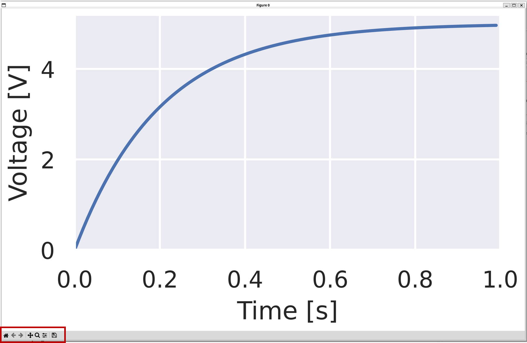
Screenshot of a figure made using matlplotlib.
The basic matplotlib syntax is fairly straightforwards, if it takes quite a few lines of code to do everything.
fig0, ax0 = plt.subplots()makes a new figure and an axis in this figure.ax0.plot(t, v)plots a line on the axis we ask for.There are then a number of commands to control the formatting of the plot.
You need to explicitly call
fig0.show()to display the plot. (This let you build up more complicated plots, and only display them when you’re ready.)Finally, we call
plt.show(). This stops the program from completing until all of the figures have been closed. Without this, the program will display the figures, and then quickly close them rather than waiting until you’ve finished looking at them. For how we’re using matplotlib here, we only want oneplt.show()at the end of the code, so further plots should be above this line.
The plot controls are in the bottom left of the figure. Try zooming in on the plot to see more detail. You can also hover over the line to see the exact values at each point. When you’re done, press the home button (the house icon) to return to the original view.
To add a second line, you just call
ax0.plot()again with the new data. A new line will automatically be added to the existing axis.Remember to call
fig0.show()to actually draw the updated plot.The code below also adds a legend to the plot, so you can tell which line is which.
# Make and plot second line
t1, v1 = make_example_signal(A=5, tau=0.1)
ax0.plot(t1, v1, linestyle="--")
ax0.legend([r"$\tau$ = 0.2 s", r"$\tau$ = 0.1 s"])
fig0.show()
Your figure should look like the below.
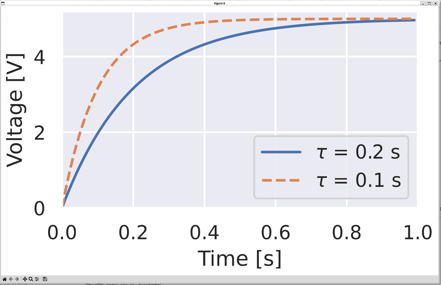
Screenshot of a figure made using matlplotlib.
By searching the Internet, asking AI, or similar, modify your plot to change the line style and markers so that it looks like the below.
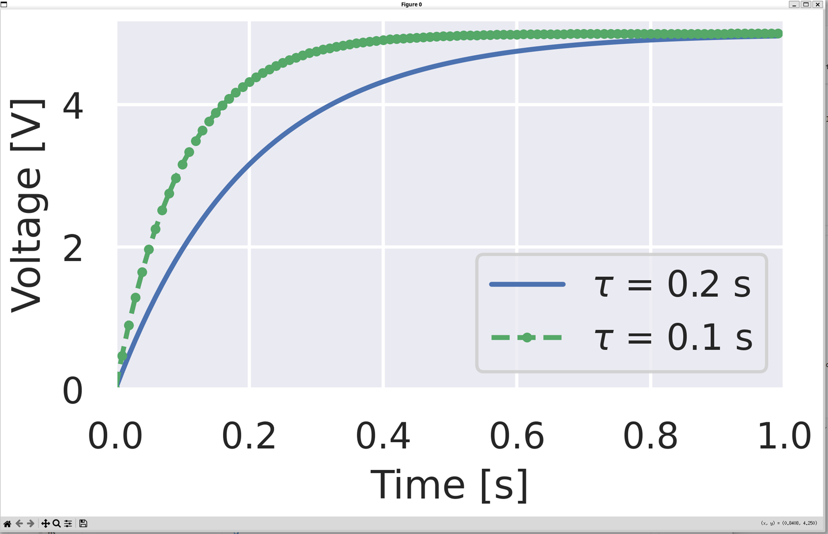
Screenshot of a figure made using matlplotlib.
Solution
In this plot, the second line is green, and uses circle symbols to mark each data point. To achieve this, change the plot command to
ax0.plot(t1, v1, color="g", linestyle="--", marker="o", markersize=2)
By searching the Internet, asking AI, or similar, add a vertical line at the time constant of each line (0.2 s and 0.1 s). You can do this using
plt.axvline().Solution
ax0.axvline(0.1, color="b", linestyle="--")
ax0.axvline(0.2, color="g", linestyle=":")
fig0.show()
Other plot types
There are many different types of plot that you might want to make. Here are a few examples using the student marks data defined above.
Copy and paste the code below into your file to plot a histogram of the course 1 marks. Remember to put this above the final
plt.show()line.# Get student marks marks_course_1, marks_course_2 = get_student_marks() # Plot histogram of student marks fig1, ax1 = plt.subplots() # make a new figure, no. 1 ax1.hist(marks_course_1) ax1.set(xlabel="Marks") ax1.set(ylabel="Number of students") fig1.show()
Copy and paste the below to make a box plot comparing the marks for course 1 and course 2. Which course did the students do generally better in?
# Plot boxplot of student marks
fig2, ax2 = plt.subplots()  # make a new figure, no. 2
ax2.boxplot([marks_course_1, marks_course_2])
ax2.set_xticklabels(["Course 1", "Course 2"])
ax2.set(ylabel="Marks")
fig2.show()
Solution
Course 1
Using
.pie()make a pie chart like the below, showing the distribution of classifications in course 1.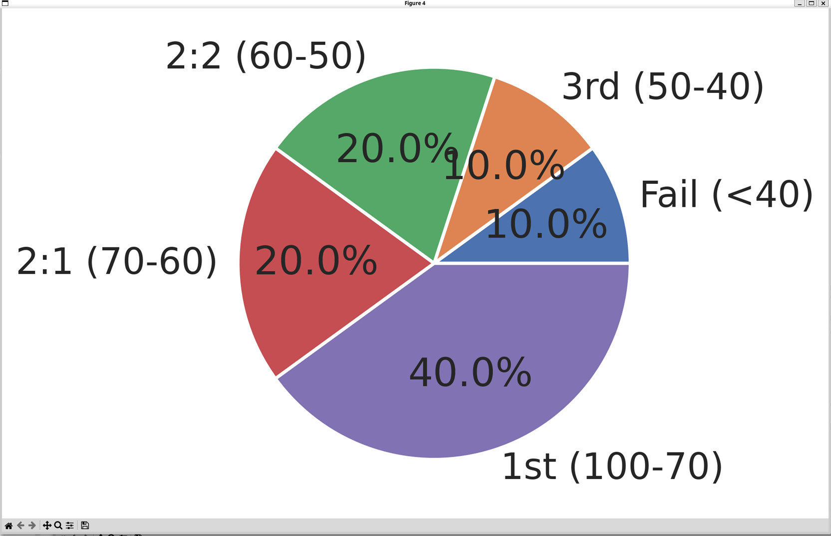
Screenshot of a figure made using matlplotlib.
Solution
# Make pie chart of student marks in course 1
fig3, ax3 = plt.subplots()  # make a new figure, no. 3
boundaries = (0, 40, 50, 60, 70, 100)
counts, _ = np.histogram(marks_course_1, bins=boundaries)
labels = [
    f"Fail (<{boundaries[1]})",
    f"3rd ({boundaries[2]}-{boundaries[1]})",
    f"2:2 ({boundaries[3]}-{boundaries[2]})",
    f"2:1 ({boundaries[4]}-{boundaries[3]})",
    f"1st ({boundaries[5]}-{boundaries[4]})",
]
ax3.pie(counts, labels=labels, autopct="%1.1f%%")
fig3.show()
There are lots of matplotlib examples online. Try some of these out.
Subplots
Having more than one plot in a figure is often useful to compare different data.
So far we’ve used plt.subplots() to make a signle figure with a single axis on it. You can also use plt.subplots() to make multiple subplots in a single figure.
The code below makes 4 subplots. The axis in each subplot is given an address,
[0,0],[0,1]and so on. We then plot, exactly as we have before, but onto the axis that we want. Copy to code below. You should get a plot like that below.# Make subplot combining existing figures fig4, axs = plt.subplots(nrows=2, ncols=2) axs[0, 0].plot(t, v) axs[0, 1].hist(marks_course_1) axs[1, 0].boxplot([marks_course_1, marks_course_2]) axs[1, 1].pie(counts, labels=labels, autopct="%1.1f%%") fig4.show()
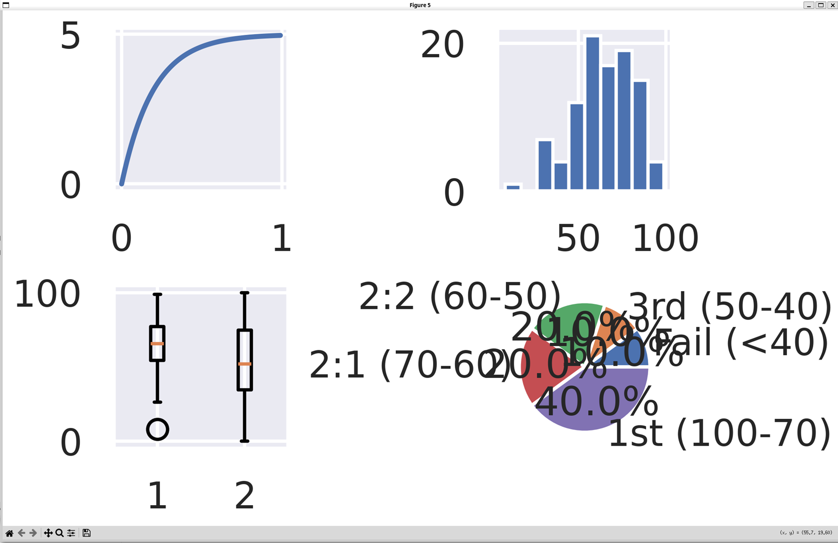
Screenshot of a figure made using matlplotlib.
We still need to add the various labels to the plots, exactly as before. The text is also too large and needs reducing. See if you can tidy the plot up.
Solution
fig5, axs = plt.subplots(nrows=2, ncols=2)
fsize = 4
axs[0, 0].plot(t, v)
axs[0, 0].plot(t1, v1, color="g", linestyle="--", marker="o", markersize=2)
axs[0, 0].axvline(0.1, color="b", linestyle="--")
axs[0, 0].axvline(0.2, color="g", linestyle=":")
axs[0, 0].set_xlabel("Time [s]", fontsize=fsize)
axs[0, 0].set_ylabel("Voltage [V]", fontsize=fsize)
axs[0, 0].legend([r"$\tau$ = 0.2 s", r"$\tau$ = 0.1 s"], fontsize=fsize)
axs[0, 0].set(xlim=(0, 1))  # set the default zoom
axs[0, 0].set(ylim=(0, 5.2))
axs[0, 0].tick_params(axis="both", labelsize=fsize)
axs[0, 1].hist(marks_course_1)
axs[0, 1].set_xlabel("Marks", fontsize=fsize)
axs[0, 1].set_ylabel("Number of students", fontsize=fsize)
axs[0, 1].tick_params(axis="both", labelsize=fsize)
axs[1, 0].boxplot([marks_course_1, marks_course_2])
axs[1, 0].set_xticklabels(["Course 1", "Course 2"], fontsize=fsize)
axs[1, 0].set_ylabel("Marks", fontsize=fsize)
axs[1, 0].tick_params(axis="both", labelsize=fsize)
axs[1, 1].pie(
    counts, labels=labels, autopct="%1.1f%%", textprops={"fontsize": fsize}
)
fig5.show()
Make a figure that looks like the below, plotting pie charts for the two sets of student marks next to one another.
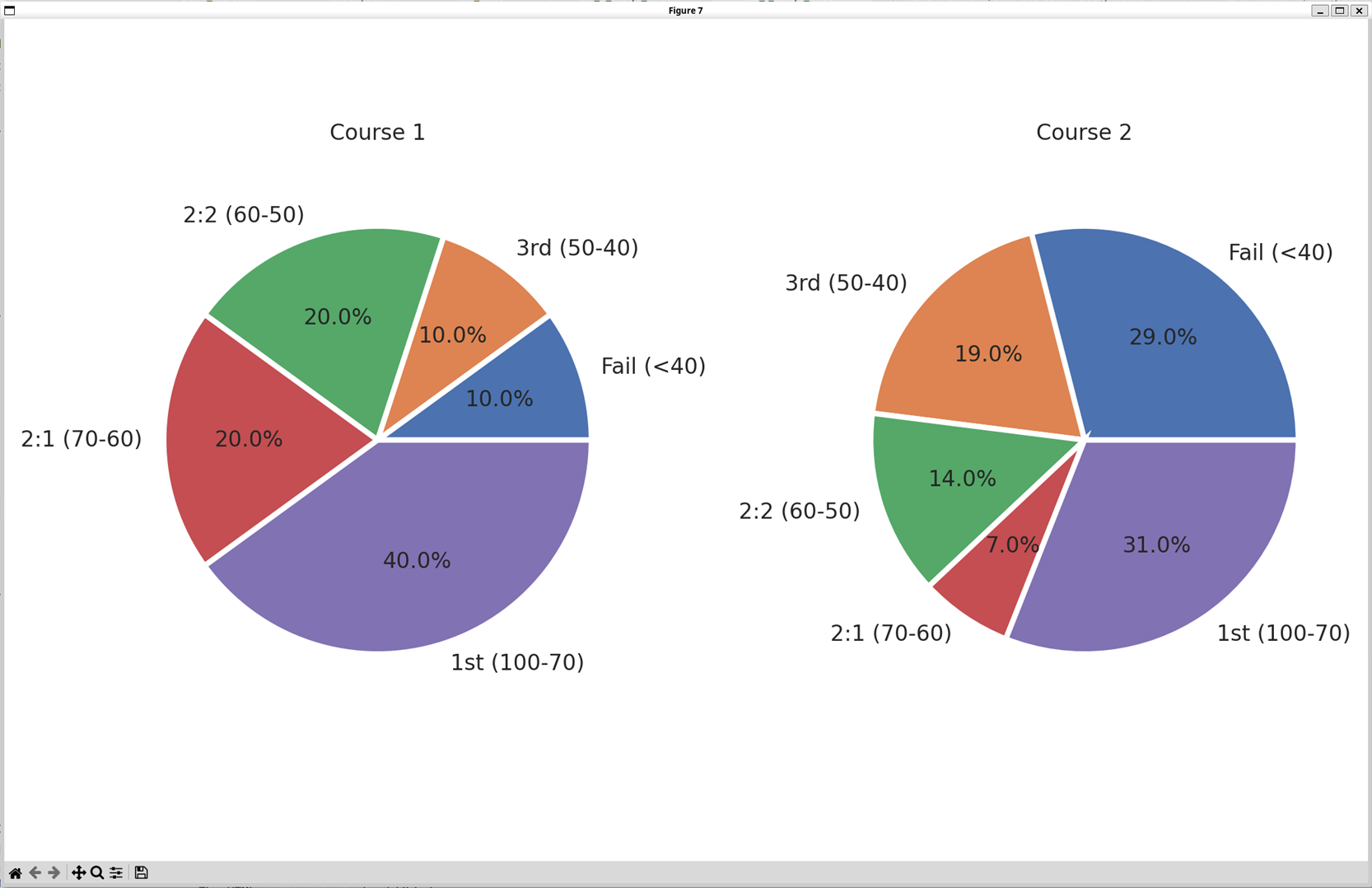
Screenshot of a figure made using matlplotlib.
Solution
# Make pie charts for both courses side by side
fig6, axs = plt.subplots(nrows=1, ncols=2)
axs[0].pie(counts, labels=labels, autopct="%1.1f%%", textprops={"fontsize": fsize})
axs[0].set_title("Course 1", fontsize=fsize)
counts_2, _ = np.histogram(marks_course_2, bins=boundaries)
axs[1].pie(
    counts_2, labels=labels, autopct="%1.1f%%", textprops={"fontsize": fsize}
)
axs[1].set_title("Course 2", fontsize=fsize)
fig6.show()
Saving plots to files
We can save a figure to a file using the .savefig() method on the figure. Run the free examples below, and compare the saved files, particularly when you zoom in. You should see that the low resolution one doesn’t look very good.
# Save figures
fig0.savefig("line_plots_low_resolution.png", dpi=60)
fig0.savefig(
    "line_plots_high_resolution.png"
)  # uses the default, set to be 600 earlier
fig0.savefig("line_plots_vector_format.pdf")
4.3.1.3. Licensing
Plotly logo is used from Wikipedia and is licensed under CC BY-SA 4.0.
Matplotlib logo is used from Wikipedia and is unlicensed material.